
Journal of Geographical Sciences >
Erosions on the southern Tibetan Plateau: Evidence from in-situ cosmogenic nuclides 10Be and 26Al in fluvial sediments
|
Zhang Xiaolong (1989-), PhD Candidate, specialized in cosmogenic nuclide applications. E-mail: xiaolong_zhang@tju.edu.cn |
Received date: 2021-02-02
Accepted date: 2021-09-14
Online published: 2022-04-25
Supported by
Second Tibetan Plateau Scientific Expedition and Research (STEP) Program(2019QZKK0707)
National Key Research and Development Program of China(2020YFA0607700)
National Natural Science Foundation of China(41930863)
China Seismic Experimental Site(2019CSES0104)
Investigating topographic and climatic controls on erosion at variable spatial and temporal scales is essential to our understanding of the topographic evolution of the orogen. In this work, we quantified millennial-scale erosion rates deduced from cosmogenic 10Be and 26Al concentrations in 15 fluvial sediments from the mainstream and major tributaries of the Yarlung Zangbo River draining the southern Tibetan Plateau (TP). The measured ratios of 26Al/10Be range from 6.33 ± 0.29 to 8.96 ± 0.37, suggesting steady-state erosion processes. The resulted erosion rates vary from 20.60 ± 1.79 to 154.00 ± 13.60 m Myr-1, being spatially low in the upstream areas of the Gyaca knickpoint and high in the downstream areas. By examining the relationships between the erosion rate and topographic or climatic indices, we found that both topography and climate play significant roles in the erosion process for basins in the upstream areas of the Gyaca knickpoint. However, topography dominantly controls the erosion processes in the downstream areas of the Gyaca knickpoint, whereas variations in precipitation have only a second-order control. The marginal Himalayas and the Yarlung Zangbo River Basin (YZRB) yielded significantly higher erosion rates than the central plateau, which indicated that the landscape of the central plateau surface is remarkably stable and is being intensively consumed at its boundaries through river headward erosion. In addition, our 10Be erosion rates are comparable to present-day hydrologic erosion rates in most cases, suggesting either weak human activities or long-term steady-state erosion in this area.
ZHANG Xiaolong , XU Sheng , CUI Lifeng , ZHANG Maoliang , ZHAO Zhiqi , LIU Congqiang . Erosions on the southern Tibetan Plateau: Evidence from in-situ cosmogenic nuclides 10Be and 26Al in fluvial sediments[J]. Journal of Geographical Sciences, 2022 , 32(2) : 333 -357 . DOI: 10.1007/s11442-022-1950-4
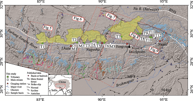
Figure 1 Shaded relief map showing sampling sites (square) in this work and sample locations (circles) in previous studies. Green squares refer to tributary samples and white squares to mainstream samples in this study; colored circles refer to basin or bedrock samples in previous studies; only tributary basins in this study are shown in light yellow. Sample IDs are consistent with those listed in Tables 1 and 2. |
Table 1 Sample information and parameters characterized for each catchment used in Figures 3 and4 -8 |
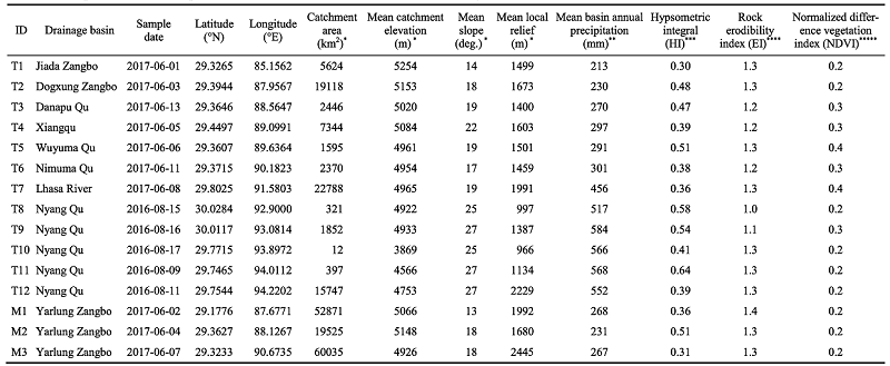 |
'Derived with the 90 m resolution SRTM DEM in ArcGIS. "Calculated from the WorldClim V. 2 monthly climate dataset (1 km2 resolution), covering precipitation from 1970 to 2000 (Fick and Hijmans, 2017). * Calculated following Perez- Pea et al. (2016).. **** Calculated based on the Global Lithological Map database (GLiM) V. 1.0 (Hartmann and Moosdorf, 2012) after Moosdorf et al. (2018). **Derived from the MODIS dataset with a spatial resolution of 500 m (https://pdaac.ugs.gov). |
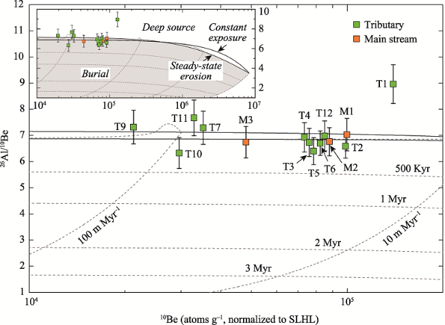
Figure 2 Plot of 26Al/10Be ratios versus 10Be concentration. To allow data from samples with different production rates to be compared on the same diagram, 10Be concentrations are normalized to sea level high latitude (SLHL). |
Table 2 Analytical results of cosmogenic radionuclide 1'Be and 26A1 for river sediments from southern Tibet |
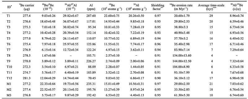 |
*ID = Sample number shown in Figure 1; T refers to tributary and M to mainstream. **"Topographic shielding factor calculated following Li (2013) with 5° in elevation angles and 10° interval in azimuth. ***"Timescale of integration for erosion (T=z*/erosion rate, with z* the mean attenuation path length; a value of 60 cm was assigned for all the samples according to Lal, 1991 and Von Blanckenburg, 2005_ ENREF 10_ENREF_14) |
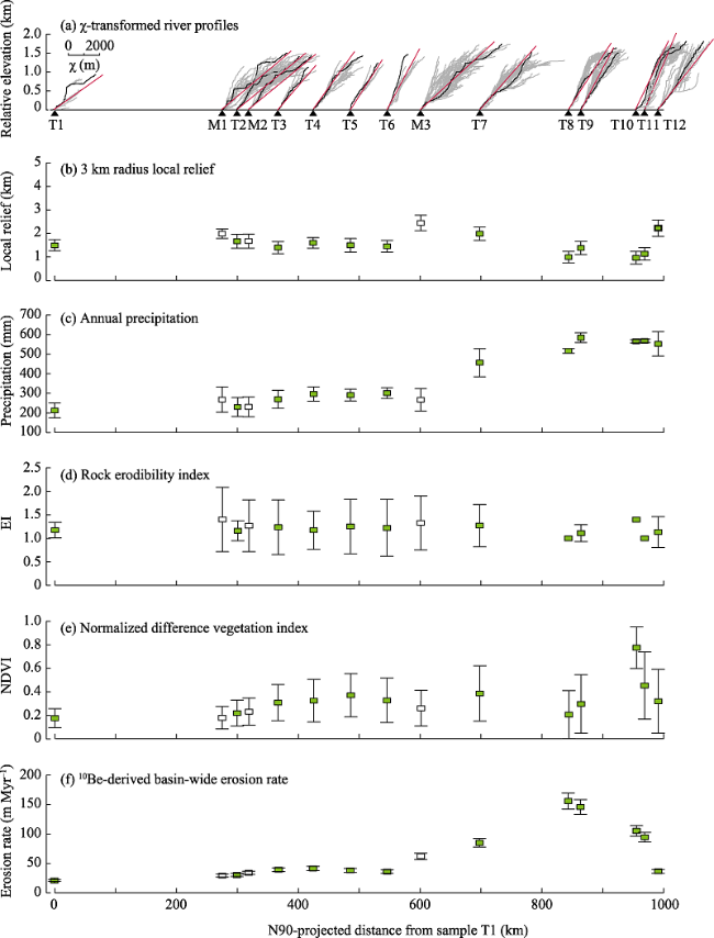
Figure 3 Characteristics of sampled basins. (a) χ-transformed river profiles, derived using TopoToolbox v2 (Schwanghart and Scherler, 2014b). The black line in each river network denotes mainstream. Corresponding tributaries are shown in grey. The red line represents the linear fitting for the drainage network. Each drainage network is positioned along the abscissa based on the N90-projected distance from their outlet to sample T1. (b) 3 km radius local relief; (c) annual precipitation; (d) rock erodibility index (EI), calculated from the Global Lithological Map (GLiM) v1.0 after Moosdorf et al. (2018); (e) normalized difference vegetation index (NDVI); and (f) 10Be-derived basin-scale erosion rate. Errors in Figures 3b-3f are reported at 1σ level. |
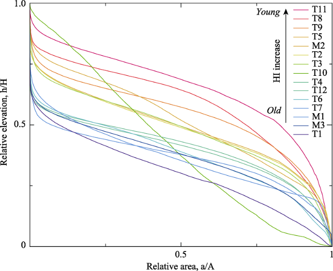
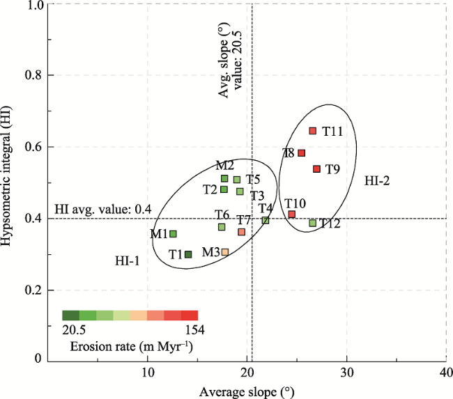
Figure 4 Hypsometric curves for the 15 drainage basins in this study. Total elevation (H) denotes the relief within the drainage basin; total area (A) denotes the total area of the drainage basin; area (a) equals to the area within the drainage basin above a certain altitude (h). Convex hypsometric curves and high HI values typically represent young and slightly eroded areas, while S- and concave-shaped curves together with low HI values characterize moderately to highly eroded areas with mature or final (old) erosional stage. The value of hypsometric integral (HI) equals to the area below the curve (Pérez-Pea et al., 2016). |
Table 3 Information about the mainstream hydrologic stations and calculated hydrologic erosion rate* |
| Station | Latitude (°N) | Longitude (°E) | Elevation (m) | Drainage area above the hydrologic station (km2) | Annual precipitation (mm) | Annual discharge (108 m3) | Annual sediment load (t km-2 yr-1) | Hydrologic erosion rate (m Myr-1) |
|---|---|---|---|---|---|---|---|---|
| Lhaze | 29.1167 | 87.5833 | 4000 | 47832 | 273 | 52 | 39.4 | 14.6 |
| Nugesha | 29.3000 | 89.7500 | 3720 | 106060 | 378 | 158 | 217.0 | 80.4 |
| Yangcun | 29.2667 | 91.8167 | 3500 | 151507 | 361 | 306 | 329.8 | 122.1 |
| Nuxia | 29.4667 | 94.6500 | 2780 | 191235 | 480 | 576 | 155.5 | 57.6 |
*Data in columns 2-8 are from Shi et al. (2018). Hydrologic erosion rates in column 9 are calculated by dividing annual sediment load with a density of 2.7 g cm-3. |
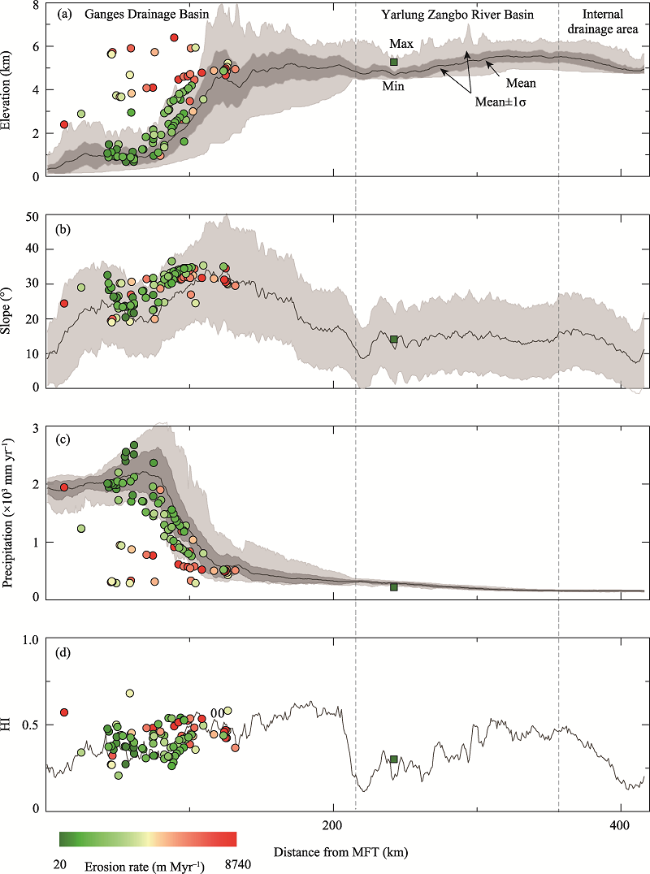
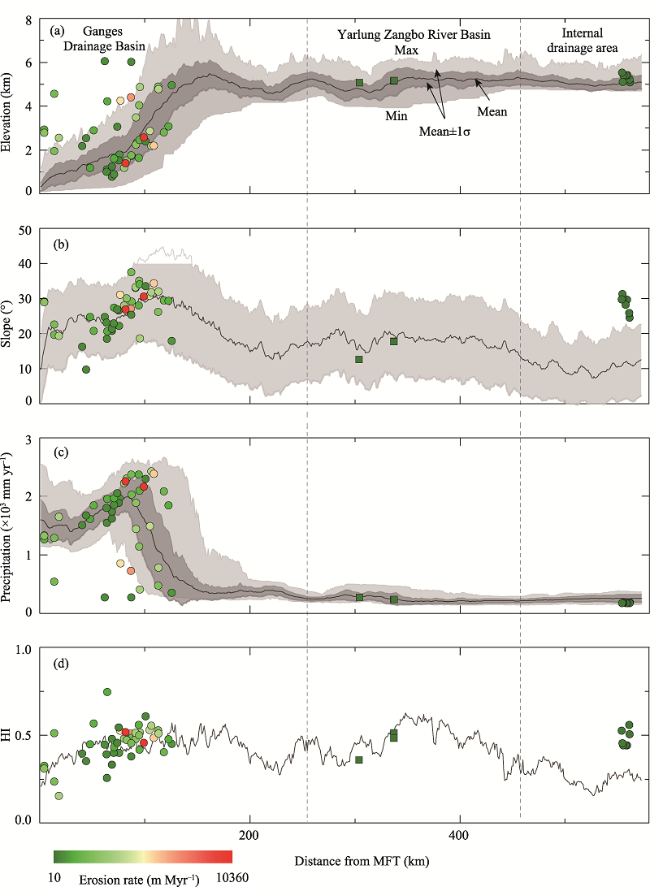
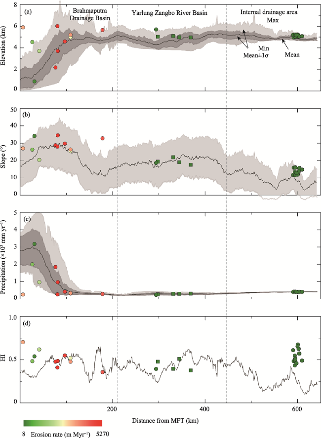
Figure 5 Swath profile from SW to NE in Figure 1, showing the variations of (a) elevation; (b) slope; (c) annual precipitation; (d) hypsometric integral (HI) for sampled basins in this paper (squares) and in previous studies (cycles). Colors of different gradient refer to erosion rate of different magnitude. |
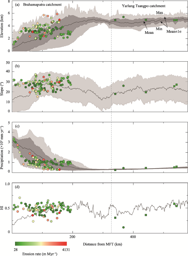
Figure 6 Swath profile from SW to NE in Figure 1: (a) elevation; (b) slope; (c) annual precipitation; (d) hypsometric integral (HI) for sampled basins in this paper (squares) and in previous studies (cycles). Colors of different gradient refer to erosion rate of different magnitudes. |
Figure 7 Swath profile from SW to NE in Figure 1: (a) elevation; (b) slope; (c) annual precipitation; (d) hypsometric integral (HI) for sampled basins in this paper (squares) and in previous studies (cycles). Colors of different gradient refer to erosion rate of different magnitude. |
Figure 8 Swath profile from SW to NE in Figure 1: (a) elevation; (b) slope; (c) annual precipitation; (d) hypsometric integral (HI) for sampled basins in this paper (squares) and in previous studies (cycles). Colors of different gradient refer to erosion rate of different magnitude. |
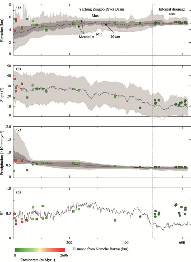
Figure 9 Swath profile from SE to NW in Figure 1: (a) elevation; (b) slope; (c) annual precipitation; (d) hypsometric integral (HI) for sampled basins in this paper (squares) and in previous studies (cycles). Colors of different gradient refer to erosion rate of different magnitude |
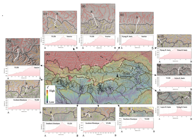
Figure 11 Map of χ' for southern Tibetan Plateau, showing geometric disequilibrium in drainage networks. Difference in χ' values between two adjacent basins can indicate the migration of basin divide and exchange of basin area. In Figures b-k, the white thick line starts from A to B and crosses the divide between basin A and basin B along the valley bottoms. The maps below Figures b-k show the variations of topography following these white thick lines. Values of χ' are inversely consistent with topographic asymmetry between basin A and basin B. |
| [1] |
|
| [2] |
|
| [3] |
|
| [4] |
|
| [5] |
|
| [6] |
|
| [7] |
|
| [8] |
|
| [9] |
|
| [10] |
|
| [11] |
|
| [12] |
|
| [13] |
|
| [14] |
|
| [15] |
|
| [16] |
|
| [17] |
|
| [18] |
|
| [19] |
|
| [20] |
|
| [21] |
|
| [22] |
|
| [23] |
|
| [24] |
|
| [25] |
|
| [26] |
|
| [27] |
|
| [28] |
|
| [29] |
|
| [30] |
|
| [31] |
|
| [32] |
|
| [33] |
|
| [34] |
|
| [35] |
|
| [36] |
|
| [37] |
|
| [38] |
|
| [39] |
|
| [40] |
|
| [41] |
|
| [42] |
|
| [43] |
|
| [44] |
|
| [45] |
Von Blanckenburg F, 2005. The control mechanisms of erosion and weathering at basin scale from cosmogenic nuclides in river sediment. Earth and Planetary Science Letters, 237(3): 462-479.
|
| [46] |
|
| [47] |
|
| [48] |
|
| [49] |
|
/
| 〈 |
|
〉 |