Special Issue: Climate Change and Its Regional Response

The response of key ecosystem services to land use and climate change in Chongqing: Time, space, and altitude

  • GAO Jie , 1, 2, 3 ,
  • BIAN Hongyan , 1, 2, * ,
  • ZHU Chongjing 1 ,
  • TANG Shuang 1
Expand
  • 1. Chongqing Jinfo Mountain Karst Ecosystem National Observation and Research Station, School of Geographical Sciences, Southwest University, Chongqing 400715, China
  • 2. Chongqing Key Laboratory of Karst Environment, School of Geographical Sciences, Southwest University, Chongqing 400715, China
  • 3. School of Geographical Sciences, State Cultivation Base of Eco-agriculture for Southwest Mountainous Land, Chongqing 400715, China
*Bian Hongyan (1986-), Lecturer, E-mail:

Gao Jie (1986-), Associate Professor, specialized in the ecosystem services, land use change. E-mail:

Received date: 2021-02-21

  Accepted date: 2021-09-17

  Online published: 2022-04-25

Supported by

National Natural Science Foundation of China(41701611)

National Natural Science Foundation of China(41830648)

General Program of Social Science and Planning of Chongqing(2020YBZX15)

Fundamental Research Funds for the Central Universities(XDJK2019C090)

Abstract

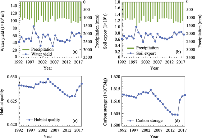
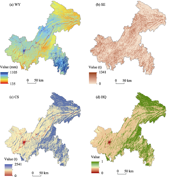
Mountainous landscapes are particularly vulnerable and sensitive to climate change and human activities, and a clear understanding of how ecosystem services (ES) and their relationships continuously change over time, across space, and along altitude is therefore essential for ecosystem management. Chongqing, a typical mountainous region, was selected to assess the long-term changes in its key ES and their relationships. From 1992 to 2018, the temporal variation in water yield (WY) revealed that the maximum and minimum WYs occurred in 1998 and 2006, which coincided with El Niño-Southern Oscillation and severe drought events, respectively. Soil export (SE) and WY were consistent with precipitation, which reached their highest values in 1998. During this period, carbon storage (CS) and habitat quality (HQ) both decreased significantly. ES in Chongqing showed large variations in altitude. Generally, WY and SE decreased with increasing altitude, while CS and HQ increased. For spatial distribution, WY and SE showed positive trends in the west and negative trends in the east. In regard to CS and HQ, negative trends dominated the area. Persistent tradeoffs between WY and soil conservation (SC) were found at all altitude gradients. The strong synergies between CS and HQ were maintained over time.

Cite this article

GAO Jie , BIAN Hongyan , ZHU Chongjing , TANG Shuang . The response of key ecosystem services to land use and climate change in Chongqing: Time, space, and altitude[J]. Journal of Geographical Sciences, 2022 , 32(2) : 317 -332 . DOI: 10.1007/s11442-022-1949-x

1 Introduction

Mountainous areas, home to 40% of the world's population, offer major benefits to humans (Mengist et al., 2020). They not only provide fiber and food products but also regulate soil, floods, and climate. The residents of such an ecosystem and those living nearby can benefit greatly when it is well protected (Gret-Regamey et al., 2008). With their unique geomorphological, hydrological, and geological features, these areas are particularly ecologically vulnerable and sensitive to climate change and human activities. The continuous provisioning of ecosystem services (ES) in mountainous areas has become increasingly challenging due to human-induced and natural changes (Balthazar et al., 2015; Schirpke et al., 2019). The persistent decrease in the capacity of mountain ecosystems to deliver services is disproportionately borne by local residents, as they tend to heavily depend on ES (MEA, 2005). Research on the spatial and temporal dynamics of ES in mountainous areas under the combined effects of land use and climate change is urgently needed.
Previous research has found that mountainous regions have a high capacity to provide regulating (e.g., climate regulation and soil conservation (SC)) and supporting ES (e.g., biodiversity protection) (Chaudhary et al., 2017; Seidl et al., 2019). Mountainous regions, with large proportions of woodlands and grasslands, have a considerably higher potential carbon stock than that observed in many other parts of the world (Erb et al., 2018). Therefore, they have been recognized as an important source in mitigating climate change (Griscom et al., 2017). These areas are also characterized by steep slopes and high relief energy, which easily cause soil loss through erosion. The SC provided by high-elevation forests is of particular relevance in mountainous regions. The forests and grasslands in mountainous regions support a large number of flora and fauna and are considered global biodiversity hotspots (Payne et al., 2017). Mountainous regions also supply fresh water for agricultural irrigation and consumption for local and downstream residents. The unique topography and landscape characteristics of mountainous regions are beneficial for the existence of diverse mountain ecosystems and likely provide multiple ES to humans (Gratzer and Keeton, 2017). Furthermore, these topographic features could lead to complex interactions between ES (Bennett et al., 2009; Wang and Dai, 2020).
Assessing the long-term changes in important ES and their relationships offers sustainable management and policy-making suggestions (Qiu et al., 2018). Previously, much research on the spatiotemporal changes of ES and their relationships was based on specific years (Sun and Li, 2017), which could lead to the loss of important information such as maximum and minimum values. The research results cannot provide more nuanced and complete information for decision-makers and stakeholders. Furthermore, altitude plays a key role in ES in mountainous regions, which has received less attention in previous studies. Located in the upper reaches of the Yangtze River, Chongqing, with a mountainous area of 62,500 km2, occupies nearly 75% of the total area (Cao and Yuan, 2019). The landscape and environment in Chongqing have experienced major changes due to climate change and socioeconomic development, which in turn can impose pressure on ES. As a mountainous region, urgent research is needed to assess how crucial ES have changed along with land use and climate change. Our research attempts to fully determine the past and current situation for important ES in Chongqing through the use of continuous data. For mountainous regions, water yield, soil conservation, carbon storage, and habitat quality are crucial for people living inside and outside this mountainous ecosystem. Based on the above context, the following steps were taken in our study: (1) to quantify continuous spatiotemporal dynamics of water yield (WY), soil export (SE), habitat quality (HQ), and carbon storage (CS) from 1992 to 2018; (2) to detect how ecosystem services change with space, time, and altitude; and (3) to analyze how ES relationships change.

2 Materials and methods

2.1 Study area

Chongqing (105°17′-110°11′E, 28°10′-32°13′N), located in southwestern China, is the newest of the four municipalities directly under the leadership of the Central Government and the largest economic center in the upper reaches of the Yangtze River, and it abounds with biological resources. The Yangtze River runs from southwest to northwest through Chongqing. As its tributary, the Jialing River joins it at the center. The total area of the region is 82,400 km2. The elevation of Chongqing ranges from 53 to 2778 m with high topographic relief (Figure 1). This region exhibits diversified geomorphic types, which include mountainous areas (75.9%), hilly areas (18.2%), and flat areas (only 5.8%). The climate is a typical subtropical monsoon climate with an annual average temperature of 17°C. The annual average precipitation is 1200 mm, with the rainy season lasting from April to September.
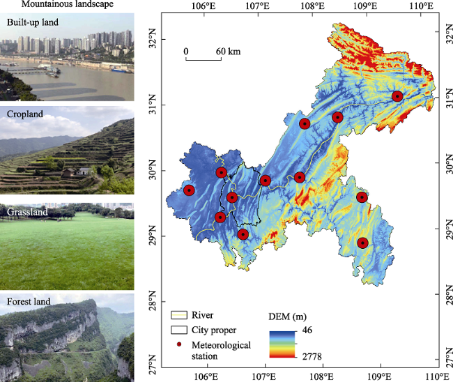
Figure 1 Elevation, meteorological stations, main rivers, and the mountainous landscape of Chongqing

2.2 Data sources

The InVEST model requires spatial map datasets and specific biophysical tables as inputs. Four types of data were analyzed in our study: (1) land-use maps, (2) climate data, (3) soil data, and (4) digital elevation model data. A detailed description of these data is given in Table 1. We validated the results of the InVEST model by comparing it with reported results from hydrological stations and previous studies (see Supplementary File A).
Table 1 Description of the datasets adopted in this study
Dataset Source Description Spatial resolution or distribution Temporal resolution
Land-use data European Space Agency http://maps.elie.ucl.ac.be/CCI/viewer/ Land use and land cover (LULC) maps on an annual basis from 1992 to 2018 300 m×300 m Yearly
Climate data China Meteorological Data Network http://data.cma.cn/ Maximum, minimum and average temperatures, precipitation, and solar radiation 12 stations
Daily/
monthly
Soil data Harmonized World Soil
Database (HWSD)
http://webarchive.iiasa.ac.at/Research/LUC/External-World-soil-database/HTML/
Soil properties including the texture, organic matter content, and root depth 30 arc-second -

2.3 Method description

2.3.1 Ecosystem services selection

The ES indicators in this study were selected based on three principles: (1) ES with high relevance in mountainous regions, (2) local stakeholder concerns, and (3) data availability. Regulating and supporting ES indicators, such as SE, CS, and HQ, are of particular relevance in mountainous regions due to their unique topography and high proportion of forests. The quantity of water discharge is particularly pertinent to the understanding of local and downstream flood and drought risks, as Chongqing is located in the upper reaches of the Yangtze River. Therefore, WY, SE, CS, and HQ were selected as the ES in this research.

2.3.2 Ecosystem services assessment

To assess the ES in our study area, we selected the InVEST model, a widely applied tool for this purpose. Four types of ES were assessed, and each of the ES was calculated using different methods (Table 2). Details on the ES assessment methods are provided in Supplementary File B.
Table 2 Methods for ecosystem service assessment
Ecosystem service indicators Methods Unit Equation References
Water yield Water balance equation m3. ha-1 ${{Y}_{x}}=\left( 1-\frac{AE{{T}_{x}}}{{{P}_{x}}} \right)\times {{P}_{x}}$
Yx: the water yield for pixel x; Px: the annual precipitation for pixel x; and ATEx: the annual actual evapotranspiration for pixel x.
(Budyko, 1974; Sharp et al., 2014)
Soil export
(inverse indicator of soil conservation)
Universal soil loss equation t.ha-1.y-1 USRLx= Rx×Kx×LSx×Cx×Px
USRLx: the average annual soil loss for pixel x; Rx: the rainfall factor for pixel x; Kx: the soil erodibility factor for pixel x; LSx: the field topography factor for pixel x; Cx: the cropping and management factor for pixel x; and Px: the factor describing the supporting conservation practices for pixel x.
(Wischmeier and Smith, 1978)
Carbon storage Sum of the carbon stored in
vegetation, litter and soil
Mg. ha-1 Cx =Cxabove+Cxbelow+Cxsoil+Cxdead
Cxabove, Cxbelow, Cxsoil and Cxdead are the aboveground carbon density, belowground carbon density, soil organic carbon density, and dead organic matter, respectively, for pixel x.
(Tappeiner et al., 2008)
Habitat quality Habitat quality model of InVEST Dimensionless
index (0-1)
${{Q}_{xj}}={{H}_{j}}\times \left( 1-D_{xj}^{z}/(D_{xj}^{z}+{{k}^{z}}) \right)$
Qx: the HQ for pixel x in land-use j; Hj: the habitat suitability of land-use type j; Dxjz: the total threat level in grid cell x of land-use type j; k: the half-saturation value; and z: normalized constant.
(Sharp et al., 2014)

2.3.3 Statistical tests for trend analysis

In this study, the Mann-Kendall (MK) test was applied to determine the trend changes in the ES in Chongqing (Mann, 1945; Kendall, 1948). The M-K test can be employed to detect not only meteorological and hydrological trends (Chen et al., 2014; Ullah et al., 2018) but also ES trends (Hao et al., 2017). It can be written as follows:
$S=\sum\nolimits_{i=1}^{n-1}{\sum\nolimits_{j=i+1}^{n}{sgn({{X}_{j}}-{{X}_{i}})}}$
where S is the standardized test statistic value, Xj and Xi represent the time series in year j and i (j>i), n is the study period, and sgn (Xj-Xi) is calculated as Eq. (2):
$sgn({{X}_{j}}-{{X}_{i}})=\left\{ \begin{align} & 1\mathop{{}}_{{}}^{{}}{{X}_{j}}>{{X}_{i}} \\ & 0\mathop{{}}_{{}}^{{}}{{X}_{j}}={{X}_{i}} \\ & -1\mathop{{}}_{{}}^{{}}{{X}_{j}}<{{X}_{i}} \\ \end{align} \right.$
In this study, the study periods n=27, and the Z value is used to conduct trend test (Eq. (3)). At 5% and 1% significance levels, the null hypothesis of no trend is rejected if |Z| > 1.96 and |Z| > 2.58, respectively. The positive Z value indicates an upward trend, and vice versa.
$Z= \begin{cases}\frac{S-1}{\sqrt{V A R(S)}} & S>0 \\ 0 \quad S=0 & \\ \frac{S+1}{\sqrt{V A R(S)}} & S< 0\end{cases}$
$VAR(S)=(n(n1)(2n+5)\sum\limits_{i=1}^{m}{{{t}_{i}}({{t}_{i}}1)}(2{{t}_{i}}+5))/18$
where m is the number of notes in the series, and ti is the width of nodes.
Sen's method was applied to calculate the actual amplitude of the changes in the four ES (Sen, 1968).
$\beta =\text{median}\left( \frac{{{x}_{j}}{{x}_{i}}}{j=i} \right)$

3 Results

3.1 Land-use change from 1992 to 2018

The land use in Chongqing notably changed from 1992 to 2018 (Figure 2). Croplands and woodlands were the two largest land-use types in Chongqing, occupying 55.9% and 37.3%, respectively, of its total area. Croplands experienced a reduction of approximately 2.1% from 1992 to 2018. A total of 9.82 × 10⁵ ha of croplands were converted into woodlands (68.2% of the decreased cropland area), grasslands (18.1% of the decreased cropland area), waterbodies (2.8% of the decreased cropland area), and built-up land (10.9% of the decreased cropland area). Built-up land increased by 332.5%, from 3.31 × 10⁴ ha in 1992 to 1.43 × 10⁵ ha in 2018. Woodlands increased by 2.6% as a result of encroachment into croplands. The increased woodland area was mainly distributed across cropland areas with slopes >25°, with little occurring in cropland areas with slopes between 15° and 25°.
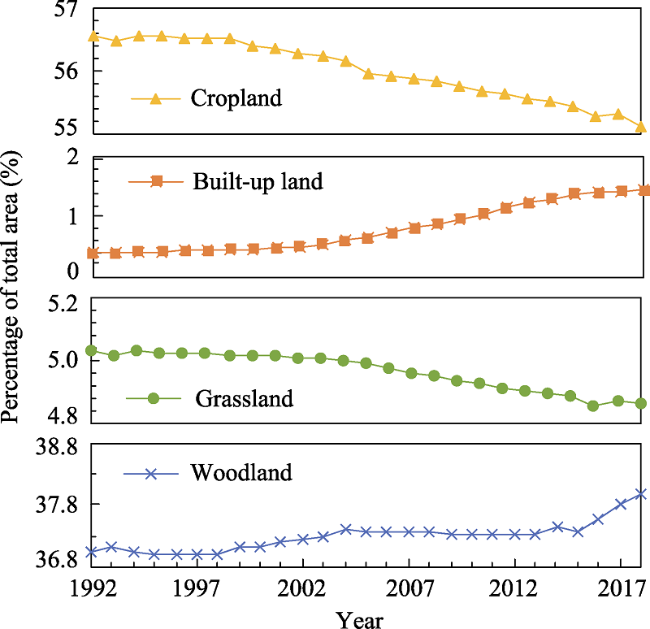
Figure 2 Trends in cropland, built-up land, grassland, and woodland changes in Chongqing from 1992 to 2018

3.2 Spatial and temporal variations in the ecosystem services

3.2.1 Temporal variation in the ecosystem services

Figure 3 shows the temporal variation in WY, SE, CS, and HQ from 1992 to 2018. WY experienced a high variation from 1992 to 2018, and the average WY was 5.37 $\times $1010 m³/a (Figure 3a). The temporal variation in WY reveals that the maximum and minimum WYs occurred in 1998 and 2006, respectively. The Mann-Kendall (MK) trend results indicate that WY showed no significant trend (Z=0.88) from 1992 to 2018. SE exhibited a similar trend to that of WY (Figure 3b). SE and WY were consistent with precipitation, which reached their highest values in 1998. The maximum and minimum SE levels occurred in 1998 and 2001, respectively. SE showed no significant trend (Z= 1.04) from 1992 to 2018.
Figure 3 Temporal variation in the ecosystem services in Chongqing from 1992 to 2018 (a. water yield; b. soil export; c. habitat quality; d. carbon storage)
Figure 3c shows the annual variation in HQ. HQ in Chongqing exhibited increasing trends from 1992 to 2004 and 2013 to 2018 and a decreasing trend from 2004 to 2013. Overall, according to the MK trend test, HQ exhibited a statistically significant negative trend (Z=–2.168). The maximum and minimum HQs occurred in 2004 and 2013, respectively. In regard to CS, a slight increase occurred from 1992 to 2004, followed by a marked decrease from 2004 to 2015 (Figure 3d). The maximum and minimum CS levels occurred in 2004 and 2015, respectively. According to the MK trend test, CS showed a significant negative trend (Z= –3.002) from 1992 to 2018 with a slope of 2.14 $\times $105 Mg/a.

3.2.2 Ecosystem services variation along altitude

WY first decreased with increasing alti-tude and then increased slightly in the high-altitude area (Table 3). The MK trend results indicate that WY showed no significant trends for any altitude gradients (|Z| < 1.96). WY showed slight upward and downward trends in different altitude gradients. SE decreased rapidly with increasing altitude and then increased slightly in high-altitude areas. SE also showed no significant trends from 1992 to 2018 for all altitude gradients, which increased and decreased slightly in different altitude gradients. Overall, CS increased with increasing altitude. The MK trend results indicated that CS showed different significant trends in different altitude gradients (|Z| > 1.96). CS showed significant decreases from 1992 to 2018 at 0-1000 m and >1500 m. HQ showed similar trends to CS.
Table 3 The average values (n=27, mean+SD) and change trends (Z values) of ecosystem services in different altitude gradients. SD represents the standard deviation.
DEM
0-500 m 500-1000 m 1000-1500 m 1500-2000 m >2000 m
Water yield 673.67±155(0.91)1 665.23 ±138(1.08) 588.81±135(0.70) 546.59±137(0.041) 560.50±144(-0.29)
Soil export 88.97±13(0.96) 88.51±12(0.91) 42.06±6(0) 23.06±3(0.29) 28.87±4(0.75)
Carbon storage 1315.17±41(-6.56) 1766.79±53(3.95) 2268.65±68(1.03) 2434.68±74(-6.59) 2380.98±72(-5.67)
Habitat quality 0.46±0.0035(-6.71) 0.64±0.0032(4.34) 0.87±0.0024(1.18) 0.95±0.0026(-6.73) 0.92±0.0034(-5.73)

1 The values in parentheses indicate the Mann-Kendall test results. The bold numbers indicate significant trends at α=0.05.

3.2.3 Spatial variation in the ecosystem services

Figure 4 shows the spatial distributions of average annual ES from 1992 to 2018. WY was higher in the southeast than in the other regions, owing to its high precipitation. Additionally, WY was also higher in central Chongqing, as it contained a higher proportion of built-up land. SE exhibited a similar pattern to that of the cropland area since agricultural activities have caused an increase in SE. Although vegetation coverage occurs in the southeast as well as in the northeast, the SE level in the former was higher because of its larger amount of precipitation and steep slopes. CS and HQ attained similar spatial distributions, which were also similar to those of the vegetation coverage. These two services decreased from east to west. Additionally, the urban areas in central Chongqing performed the worst in terms of CS and HQ, owing to numerous human activities.
Figure 4 Spatial distributions of average annual ecosystem services in Chongqing from 1992 to 2018 (WY: water yield; SE: soil export, CS: carbon storage; HQ: habitat quality)
Figure 5 shows the spatial distribution of the four ES trends according to the MK trend test results. WY showed positive trends in the west and negative trends in the east (Figure 5a). The trend analysis of SE revealed an increasing (decreasing) trend in 15 (21) counties. The spatial distribution of the SE trends exhibited a similar spatial pattern to that of the WY trends, as positive trends were observed in the west with negative in the east (Figure 5b). In regard to CS and HQ, negative trends dominated across the whole area (Figures 5c and 5d, respectively). The trend analysis of CS and HQ revealed that 7 (31) counties exhibited positive (negative) trends. According to the test results, 5 counties showed significant positive trends, while 29 exhibited significant negative trends.
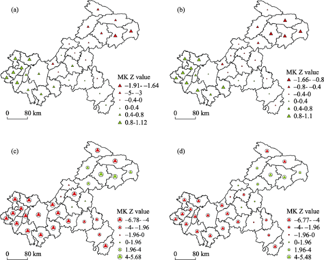
Figure 5 Spatial distribution of the annual ecosystem service trends in Chongqing from 1992 to 2018 (a. water yield; b. soil export; c. carbon storage; d. habitat quality). The black circles indicate significant trends at α=0.05. MK refers to the Mann-Kendall test.

3.3 Variation in the relationships between the ecosystem services

We performed Pearson's correlation analysis grid by grid between the ES from 1992 to 2018, which derived both the correlation coefficient (r-value) and significant value (P value). All pairs of ES were significantly correlated (P<0.01). From 1992 to 2018, the ES relationships showed interannual variations to a certain degree (Figure 6). WY and SC (inverse indicator of SE) exhibited a consistent negative relationship from 1992 to 2018, and they were weakly correlated (Pearson coefficient; 0≤ |r| < 0.3) (Figure 6b). WY showed significant negative correlations with HQ and CS (Figures 6a and 6c). The relationships for these two pairs of ES showed high interannual variations. WY was highly correlated with HQ and CS for certain years (Pearson coefficient; |r| ≥0.5). SC showed moderate synergies with HQ and CS from 1992 to 2018 (Pearson coefficient; 0.3≤ |r| < 0.5) (Figures 6d and 6e). CS and HQ exhibited a persistent notable positive relationship (Pearson coefficient; |r| ≥0.5) (Figure 6f). Furthermore, the strength of the relationship intensified over time.
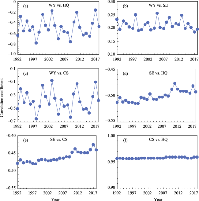
Figure 6 Variations in the relationships between the ecosystem services in Chongqing from 1992 to 2018 (WY: water yield; SE: soil export; CS: carbon storage; HQ: habitat quality). WY vs. HQ indicates the relationship between water yield and habitat quality. Y-axis represents the Pearson correlation coefficient.
The relationships for six pairs of ES at different altitude gradients were also analyzed by performing Pearson's correlation analysis grid by grid (Figure 7). Persistent tradeoffs between WY and SC were found at all altitude gradients, indicated by positive correlations between WY and SE. In addition, these two ES were weakly correlated at low altitudes and moderately correlated at high altitudes. Persistent tradeoffs between WY and HQ were found at all altitude gradients. This tradeoff intensified with increasing altitude. For relationships between WY and CS, no clear patterns were detected at low altitudes. Their relationships shifted between positive and negative over time with interannual variations. CS showed tradeoffs with WY at an altitude >500 m. Furthermore, this tradeoff intensified with increasing altitude. The relationships of SC vs. CS and SC vs. HQ remained consistently positive across all altitude gradients. However, these relationships were highly variable with altitude variations. The strength of these positive relationships increased with increasing altitude. HQ and CS were highly related at all altitude gradients. However, this synergy declined at low altitudes.
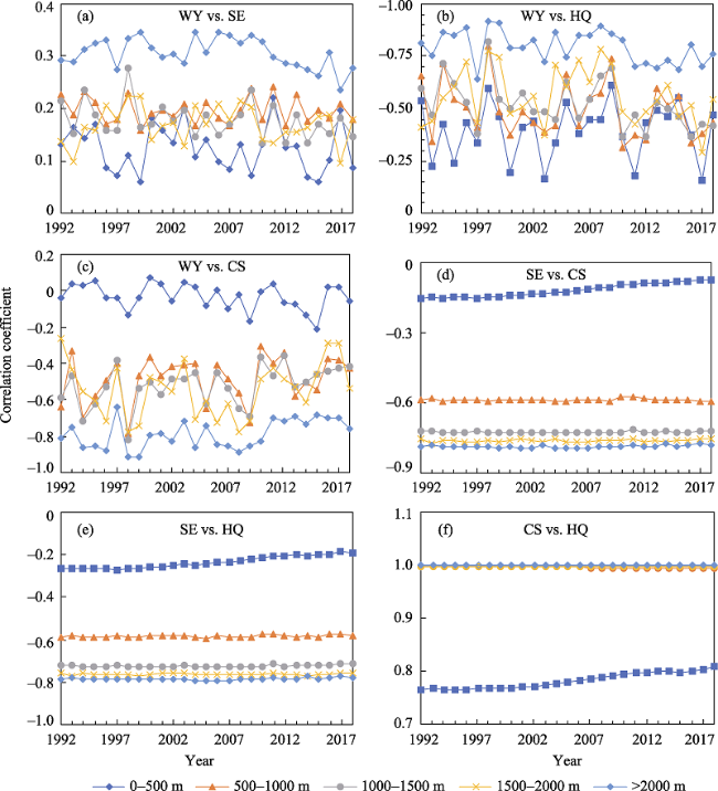
Figure 7 Variations in the relationships between the ES at different attitude gradients in Chongqing. WY vs. HQ indicates the relationship between water yield and habitat quality. Y-axis represents the Pearson correlation coefficient.

4 Discussion

4.1 Drivers of change in the ecosystem services

The selected ES experienced high interannual variations from 1992 to 2018 in our study area. Chongqing has experienced major changes in its environment and landscape due to its implementation of ecological projects, socioeconomic development, and climate change (Figures 8a and 8b). Climate factors, especially precipitation, impose a great impact on WY and SE (Zhao et al., 2017). A previous study found that precipitation could explain 80% of the annual discharge variance in the Yangtze River (Chen et al., 2014). As a key region in its upper reaches, the spatiotemporal variations in WY and SE were consistent with those in precipitation. For example, the maximum WY values in 1998 are significantly correlated with the appearance of the El Niño-Southern Oscillation (ENSO) event in April 1997. In addition, the severe drought events in 2001 and 2006 resulted in lower WY values from 1992 to 2018. Our results also have shown that climate change has a greater impact than land use change on annual WY and SE. We analyzed the discreteness of precipitation and land use by calculating their standard deviations (SD) and coefficients of variation (CV) (Table 4). Except for built-up land, the temporal variability of precipitation was higher than that of land use, as precipitation has higher coefficients of variation. Thus, temporal variations in WY and SE have emphasized the effects of temporal variability in precipitation.
The minimum WY value occurred in 2006, while the lowest precipitation was observed in 2001. This occurred because the woodlands in Chongqing have increased since 1999 due to the implementation of the Natural Forest Conservation Program (NFCP) and the Grain for Green Program (GFGP) (Figure 8a) (Liu et al., 2008). The conversion of croplands on steep slopes into woodlands could reduce WY, as canopy evapotranspiration and interception consume much of the precipitation (Gao and Bian, 2019). Our research also found that WY and SE exhibited negative trends in eastern Chongqing. Southeast and northeast Chongqing were considered important ecological conservation regions under the implementation of the GFGP in the municipality. Vegetation restoration is an effective way to reduce WY and SE as vegetation intercepts rainfall and increases infiltration (Wei et al., 2009).
Table 4 Basic statistical properties of precipitation and different land use types in Chongqing
Annual average (mm) SD2 (mm) CV2 (%)
Precipitation 1122 144 12.8
Annual average (km2) SD (km2) CV (%)
Cropland 46067 486 1.0
Woodland 30724 197 0.6
Grassland 4083 55 1.3
Built-up land 718 359 50.0
Water bodies 804 7 0.7

2 SD represents the standard deviation, and CV represents the coefficient of variation.

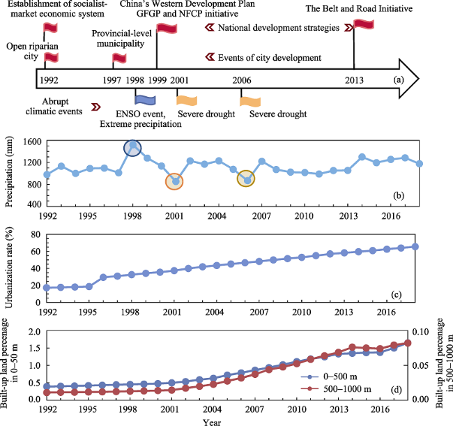
Figure 8 Major socioeconomic, policy, and climate events influencing ES in Chongqing during 1992-2018 (a, b). The urbanization rate from 1992 to 2018 is shown in the middle graph (c). Trends of the built-up land change at low altitudes (d).
In contrast to WY and SE, CS and HQ exhibited stronger responses to land-use change than to climate change (Langerwisch et al., 2018). CS and HQ first increased and then decreased, with the highest value occurring in 2004. The amount of carbon stored in vegetation varies due to woodland and grassland changes (Erb et al., 2018). Woodlands increased rapidly before 2004 and then slowly decreased, while grasslands experienced a persistent decline. Chongqing experienced rapid urbanization, as a series of socioeconomic events occurred from 1992 to 2018 (Figure 8a). For instance, Chongqing's urbanization rate has increased from 31% to 65.5% since it became China's fourth municipality in 1997 (Figure 8c). Rapid urbanization always brings along landscape change, such as the expansion of built-up areas. Despite its small proportion of the total area, built-up areas imposed a disproportionate effect on HQ degradation and the loss of terrestrial carbon stored in the vegetation biomass (Seto et al., 2012; Liu et al., 2019). Our research found that CS and HQ showed negative trends in western Chongqing. This region has experienced rapid landscape urbanization due to its relatively low and flat terrain. The changes in woodland, grassland, and urban areas in Chongqing caused variations in CS and HQ.
ES provided by mountain regions at different altitude gradients showed large variations due to differences in vegetation types and soil and climate conditions. Climate conditions such as precipitation and temperature varied with altitude, resulting in different water yields. Furthermore, the distribution of land-use types varied with altitude. Forests were mainly concentrated at high altitudes, resulting in low WY and SE, and this also led to high values of CS and HQ. The trends of ES changes also varied with altitude (Yu et al., 2021). The increased built-up areas were mainly concentrated at relatively low altitudes, which had significant negative impacts on CS and HQ (Figure 8d).

4.2 Drivers of change in the ecosystem services relationships

From 1992 to 2018, the ES relationships in Chongqing were not static. WY and SE are both affected by precipitation. High levels of precipitation will increase WY and SE at the same time. Therefore, there was a clear positive relationship between WY and SE, as they share a common driver (i.e., precipitation). The tradeoffs between WY and SC intensified at high altitudes. Vegetation coverage was the dominant factor simultaneously influencing multiple ES changes at high altitudes. Maintaining a high proportion of woodlands at high altitudes enhanced CS and HQ and had obvious effects on SE and WY reduction (similar to Sun et al., 2018; Yu et al., 2021). Therefore, the negative relationships of WY vs. CS and WY vs. HQ were strengthened at high altitudes, and the degrees of synergies between SC and HQ and CS were the highest in the same. The persistent synergies between CS and HQ indicated that an increased CS implied a higher vegetation coverage, which could help improve habitat provisions (Qiu et al., 2018).

4.3 Management and policy implications

The above results offer management and policy implications. First, the ES were uneven with high interannual variations. The water-related services (WY and SC) were especially highly associated with climate effects (e.g., precipitation). Therefore, decision-makers and managers need to consider the impact of extreme climatic events and implement corresponding measures. Second, the intense synergies between SC, HQ, and CS at high altitudes suggest that the implementation of afforestation policy and management (e.g., GFGP) in these areas may lead to great improvements in SC, HQ, and CS simultaneously. Our results offer information to managers on which of the ES relationships are probably sensitive to changes in climatic factors and which might remain robust and predictable over time (Qiu et al., 2018). For instance, the synergies between CS and HQ over time suggest that the land-use management responses may lead to similar synergistic outcomes. Local governments should establish long-term monitoring programs to reveal how the ES and their relationships change over time and across space. In particular, the long-term impacts of ecological restoration programs on ES relationships should be monitored and assessed since a previous study found that the GFGP may lead to the intensification of ES tradeoffs (Li et al., 2021).

4.4 Limitations and future studies

Our research has its limitations. Our research has only assessed four important ES, i.e., WY, SC, HQ, and CS, due to a lack of data sources. In fact, mountainous regions, which often have attractive landscapes, could provide many cultural ES to tourists and local residents (Schirpke et al., 2016). In a future study, we need to assess all ES to reflect the overall spatiotemporal changes in the ES caused by socioeconomic development, land-use policy, and climate change. Furthermore, we should assess the individual contributions of land use and climate change to ES variations, especially for water-related services. Finally, the prediction of long-term effects on natural and anthropogenic drivers of ES should be analyzed by offering a range of land-use and climate scenarios.

5 Conclusions

Our study has produced several important findings on the past and current situations for four critical ES and their relationships in Chongqing by using available continuous data. WY experienced a high variation and showed no significant trend from 1992 to 2018. SE exhibited a temporal trend similar to that of WY. The temporal changes in the water-related ES (WY and SC) were consistent with those in the precipitation. The temporal changes in water-related services have shown a much greater response to climate change than land use change, as the temporal variability of precipitation is higher than that of land use. CS and HQ revealed overall significant negative trends with increasing trends from 1992 to 2004 and 2013 to 2018 and a subsequent decreasing trend from 2004 to 2013. They have similar spatiotemporal distribution variations, which are also similar to those of vegetation coverage. WY and SE first decreased with increasing altitude and then increased slightly in the high-altitude area. The MK trend results indicate that WY and SE showed no significant trends for all altitude gradients. CS and HQ increased significantly with increasing altitude due to the increase in vegetation coverage. The relationships among the ES in Chongqing also exhibited high interannual variations to a degree, especially the relationships between the water-related and other services. The relationship between CS and HQ was robust over time and altitude. Our results provide an opportunity to manage CS and HQ simultaneously, as they exhibit persistent synergies.

Supplementary File A

Validations of water yield, soil export, carbon storage and habitat quality

1 Water yield

Chongqing government has reported the value of water yield based on the observed data from hydrological stations for ten years. We compared our simulated results with the reported data published by local government (Figure A1). After analyzing the correlation between the modeled and observed values, the results indicated that the modeled and observed values showed a perfect linear regression, with R2 and correlation coefficient values of 0.82 and 0.81 (n=10). Therefore, we considered that the simulation results for water yield in this study can present the actual results.
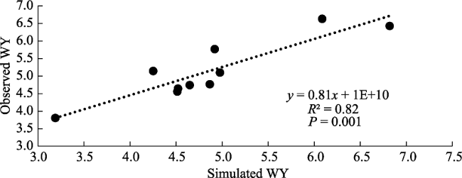
Figure A1 The observed water yield versus simulated water yield (1010 m³/a)

2 Soil export

Soil export in 2014 has been reported by Chongqing government. We only used the reported data in 2014 to validate due to the data absence of other years. Fortunately, soil export in 2014 was reported at county scale. We calculated simulated soil export at county scale and compared with reported data (Figure A2). After analyzing the correlation between the modeled and observed values, the results indicated that the modeled and observed values showed a good linear regression, with R2 and correlation coefficient values of 0.61 and 1.2 (n=38). Therefore, we considered that the simulation results for soil export in this study can present the actual results.
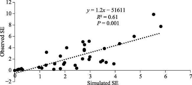
Figure A2 The observed soil export versus simulated soil export (105 t/a)

3 Carbon storage

We only obtained observed surface soil organic carbon (SSOC) of six counties in Chongqing for 2009 due to the absence of local studies (Bao et al., 2015). We calculated the soil organic carbon (SOC) as Meng (2012) found that the SSOC in 0-20 cm layer accounts for about 34% to 47% to SOC in 0-100 cm layer. After extracting the simulated SOC of the same six counties in Chongqing, validation of soil carbon storage was conducted by comparing with observed data. We analyzed the correlation between the simulated and observed values (Figure A3). The results indicated that the modeled and observed values for soil export had a perfect linear regression, with R2 and correlation coefficient values of 0.81 and 0.94 (n=6). Therefore, we considered that the simulation results for carbon storage in this study can present the actual results.
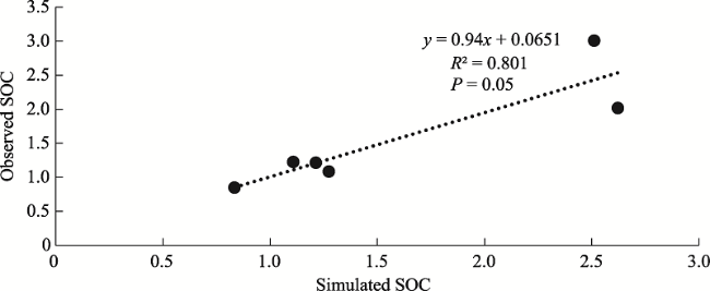
Figure A3 The observed soil organic carbon versus simulated soil organic carbon (107 t/a)

4 Habitat quality

Habitat quality depends on the intensity of external stress from threats and the relative sensitivity of habitat types to each threat. As the habitat quality index cannot be observed directly, it is hard to validate the simulated results. To improve the accuracy of results, input parameters used in our study were obtained from previous study in mountain region (Sun and Li, 2017). The properties of threats and sensitivity of habitat types to each threat in Chongqing were listed in Tables A1 and A2.
Table A1 Threats and their maximum distance of influence and weights
Threats MAX_DIST WEIGHT DECAY
Express way 8.0 0.5 Exponential
Highway 10 0.5 Exponential
Railway 7 0.7 Exponential
Urban area 10 1 Exponential

MAX_DIST: the maximum distance over which each threat affects habitat quality

WEIGHT: the impact of each threat on habitat quality, relative to other threats.

DECAY: the type of decay over space for the threat.

Table A2 The sensitivity of habitat types to each threat
NAME HABITAT Express way Highway Railway Urban area
Woodland 1.00 0.7 0.6 0.7 0.7
Grassland 0.60 0.7 0.9 0.8 0.75
Built-up land 0 0 0 0 0
Cropland 0.40 0.4 0.3 0.6 0.5
Water bodies 0.7 0.5 0.6 0.5 0.7

NAME: the name of each land use/land cover type.

HABITAT: assign each land use/land cover type a relative habitat suitability score from 0 to 1 where 1 indicates the highest habitat suitability.

References
Bao L R, Yan M S, Jia Z M et al., 2015. The distribution of the surface soil organic carbon storage and density in western Chongqing. Geophysical and Geochemical Exploration, 39(1): 180-185. (in Chinese)
Meng Y, 2012. Reserves estimation and spatial distribution of soil organic carbon in small watershed scale [D]. Wuhan: Huazhong Agricultural University. (in Chinese)
Sun X, Li F, 2017. Spatiotemporal assessment and trade-offs of multiple ecosystem services based on land use changes in Zengcheng, China. Science of The Total Environment, 609: 1569-1581.

Supplementary File B

Methods for ecosystem services assessment

1 Water yield

Water yield represents the water provisioned from all land use types. The model follows the principle of water balance, considering the interaction between climate factors and water cycle, and we obtain a distribution of the regional water yield. Water yield model is based on annual average precipitation and the Budyko curve. The yield of the grid i in the land use type j, Yij (mm/yr), is calculated as follows:
${{Y}_{ij}}=\left( 1-\frac{AE{{T}_{ij}}}{{{P}_{i}}} \right)\cdot {{P}_{i}}$
where AETij (mm/yr) is the actual evapotranspiration of grid i in the land use type j, Pi (mm/yr) is annual precipitation of raster i.
For vegetated land use/land cover (LULC), the evapotranspiration portion of the water balance, $\frac{AE{{T}_{ij}}}{{{P}_{i}}}$, is based on an expression of the Budyko curve.
$\frac{AE{{T}_{ij}}}{{{P}_{i}}}=1+\frac{PE{{T}_{ij}}}{{{P}_{i}}}-{{\left[ 1+{{\left( \frac{PE{{T}_{ij}}}{{{P}_{i}}} \right)}^{\omega i}} \right]}^{\frac{1}{\omega i}}}$
where PETij is the potential evapotranspiration and ωi is a non-physical parameter that characterizes the natural climatic-soil properties. PETij is defined as:
$PE{{T}_{ij}}={{k}_{ij}}\cdot E{{T}_{0,i}}$
where ET0,i is the reference evapotranspiration from pixel i and kij is the vegetation evapotranspiration coefficient associated with the pixel i on the land use type j.
$E{{T}_{0}}=0.0013\times 0.408\times RA\times ({{T}_{av}}+17)\times {{(TD-0.0123\times P)}^{0.76}}$
where RA is extraterrestrial radiation, Tav is the average of daily maximum and minimum temperature, TD is the difference between the average of daily maximum and minimum temperatures, and P is the monthly precipitation.
${{\omega }_{i}}=Z\cdot \frac{AW{{C}_{i}}}{{{P}_{i}}}+1.25$
$AW{{C}_{i}}=Min\text{ }(Rest\_layer\_dept{{h}_{i}},\ Root\_dept{{h}_{i}})\cdot PAW{{C}_{i}}$
where ωi is a non-physical parameter that characterizes the natural climatic-soil properties for pixel i; Z is a dimensionless constant, ranging from 1 to 30, that captures the local precipitation pattern and hydrogeological characteristics; AWCi (mm) is the volumetric plant available water content; the 1.25 term is the minimum value of ωi; and PAWC (mm) is the plant available water capacity.
For non-vegetated LULC (e.g., water, construction land), the actual annual evapotranspiration is computed directly from the reference evapotranspiration and has an upper limit defined by the precipitation:
$AE{{T}_{ij}}=Min\text{ }({{k}_{ij}}\cdot E{{T}_{{{0}_{i}}}},{{P}_{i}})$
where Pi (mm/yr) is the annual precipitation for pixel i. Parameters used for water yield can be found in Table B1.

2 Soil conservation

The universal soil loss equation (USLE) was used to evaluate soil conservation. A decrease in soil loss implies an improvement in soil conservation. We predicted the rate of soil loss for each pixel on the landscape i using Eq. (8).
$USL{{E}_{i}}={{R}_{i}}\cdot {{K}_{i}}\cdot L{{S}_{i}}\cdot {{C}_{i}}\cdot {{P}_{i}}$
where USRLi (ton·(ha·yr)-1) is the average annual soil loss for pixel i; Ri (MJ·mm·(ha·hr)-1) is the rainfall factor for pixel i; Ki (ton·ha·hr·(MJ·ha·mm)-1) is the soil erodibility factor for pixel i; LSi is the field topography factor for pixel i; Ci is the cropping and management factor for pixel i, and Pi is the factor for supporting conservation practices for pixel i.
Rainfall erosivity (R), which reflects the potential capacity of rainfall to cause erosion, is determined by a combination of the kinetic energy and intensity of rainfall. Based on rainfall data availability, this study applied R value calculations from 1992 to 2015 using monthly average rainfall (Eq. 9).
$R=\sum\limits_{n=1}^{12}{(-2.6398+0.3046\times {{p}_{n}})}$
where Pn is the total rainfall (mm) in month n.
Soil erodibility (K) is defined as the amount of eroded soil per unit area caused by rainfall erosivity, and it reflects differences in soil erosion rates when other factors that influence erosion are constant. This study used the formula from the Erosion Productivity Impact Calculator (EPIC) for this calculation (Eqs. 10-14).
${{K}_{{}}}=(-0.01383+0.51575{{f}_{csand}}\times {{f}_{cl-si}}\times {{f}_{orgc}}\times f{}_{hisand})\times 0.1317$
${{f}_{csand}}=0.2+0.3\times \exp \left[ -0.0256\times {{m}_{s}}\cdot \left( 1-\frac{{{m}_{silt}}}{100} \right) \right]$
${{f}_{cl-si}}={{\left( \frac{{{m}_{silt}}}{{{m}_{c}}+{{m}_{silt}}} \right)}^{0.3}}$
${{f}_{orgc}}=1-\frac{0.25\times {{\rho }_{orgc}}}{{{\rho }_{orgc}}+\exp \left[ 3.72-2.95\times {{\rho }_{orgc}} \right]}$
${{f}_{hisand}}=1-\frac{0.7\times \left( 1-\frac{{{m}_{s}}}{100} \right)}{\left( 1-\frac{{{m}_{s}}}{100} \right)+\exp \left[ -5.51+22.9\times \left( 1-\frac{{{m}_{s}}}{100} \right) \right]}$
where K is the soil erodibility factor; ms, msilt, mc, and ρorgc are the mass-based percentages of sand, silt, clay, and organic carbon, respectively. Parameters used in soil conservation can be found in Table B1.
Table B1 Parameters for water yield and soil conservation in Chongqing
LULC_desc Kc root_depth usle_c usle_p LULC_veg
Cropland 0.65 2100 0.25 0.4 1
Woodland 1.1 7000 0.003 1 1
Grassland 0.58 2600 0.04 0.8 1
Urban area 0.3 500 0 0 0
Water bodies 1 1000 0 0 0

LULC_desc: Descriptive name of land use/land cover class.

Kc: The plant evapotranspiration coefficient for each LULC class.

root_depth (mm): The maximum root depth for vegetated land use classes.

usle_c: Cover-management factor for the USLE. This factor is used to measure the inhibitory effect of vegetation cover and management on soil erosion.

usle_p: Support practice factor for the USLE. It is the ratio of soil loss with a support practice, such as contouring, stripping, or terracing to soil loss with straight-row farming up and down the slope.

LULC_veg: Values should be 1 for vegetated land use types except wetlands, and 0 for all other land use types, including urban, water bodies, etc.

3 Carbon storage

Regional carbon storage is closely related to the productivity and climate regulation capacity of terrestrial ecosystems. It is composed of four elements: aboveground carbon storage, belowground carbon storage, soil organic carbon storage, and dead organic matter carbon storage. Using maps of land use and land cover types, and data on the amount of carbon stored in carbon pools, this model estimates the net amount of carbon stored in a land parcel over time:
${{C}_{x}}=C_{x}^{above}+C_{x}^{below}+C_{x}^{soil}+C_{x}^{dead}$
where Cx is the total amount (Mg/ha) of carbon storage; $~C_{x}^{above},$ $\text{ }\!\!~\!\!\text{ }C_{x}^{below}$, $C_{x}^{soil}$, and $C_{x}^{dead}$ represent the amount (Mg/ha) of carbon stored in aboveground biomass, belowground biomass, soil, and dead organic matter, respectively. The biomass carbon stocks per unit area of each land use type assessed in this study were listed in Table B2 (Wang et al., 2018).
Table B2 Parameters for carbon storage in Chongqing
Items Cropland Woodland Grassland Built-up land Water bodies
Aboveground (Mg/ha) 19.5 35 15.1 0 0
Belowground (Mg/ha) 45.5 85.1 67.5 0 0
Soil organic (Mg/ha) 72.4 140.6 100 1.8 0
Dead organic (Mg/ha) 2.5 30.5 1 0 0

4 Habitat quality

Habitat quality (HQ) refers to the ability of an ecosystem to provide suitable conditions for the persistence of individuals and populations. HQ was measured by considering the intensity of external stress from threats and the relative suitability of each LULC type to each threat. The HQ score can be expressed as:
${{Q}_{xj}}={{H}_{j}}\times \left( 1-\frac{D_{xj}^{z}}{\left( D_{xj}^{z}+{{k}^{z}} \right)} \right)$
where Qxj is the HQ for pixel x in land use j, which is dimensionless. Hj is the habitat suitability of land use type j, $D_{xj}^{z}$ is the total threat level in grid cell x in land use type j, k is the half-saturation value, and z is a normalized constant. Qxj ranges from 0 to 1, with a higher score indicating a higher quality. The specific parameters used in this study can be found in Table B3 in Supplementary File B.
Table B3 Parameters for habitat quality in Chongqing
Threats
Habitat Express way Highway Railway Urban area
Properties of threats Weight - 0.5 0.5 0.7 1
Maximum distance of influence - 8 10 7 10
Sensitivity of different land cover types Woodland 1 0.7 0.6 0.7 0.7
Grassland 0.5 0.7 0.9 0.8 0.75
Built-up land 0 0 0 0 0
Cropland 0.4 0.4 0.3 0.6 0.5
Water bodies 0.7 0.5 0.6 0.5 0.7
References
Wang J Q, Zhang T, Gou J et al., 2018. Spatial-temporal changes of urban areas and terrestrial carbon storage in the Three Gorges Reservoir in China. Ecological Indicators, 95: 343-352.
[1]
Balthazar V, Vanacker V, Molina A et al., 2015. Impacts of forest cover change on ecosystem services in high Andean Mountains. Ecological Indicators, 48: 63-75.

DOI

[2]
Bennett E M, Peterson G D, Gordon L J, 2009. Understanding relationships among multiple ecosystem services. Ecology Letters, 12(12): 1394-1404.

DOI PMID

[3]
Budyko M I, 1974. Climate and Life. San Diego, CA, USA: Academic Press.

[4]
Cao W, Yuan X, 2019. Region-county characteristic of spatial-temporal evolution and influencing factor on land use-related CO2 emissions in Chongqing of China, 1997-2015. Journal of Cleaner Production, 231: 619-632.

DOI

[5]
Chaudhary S, Tshering D, Phuntsho T et al., 2017. Impact of land cover change on a mountain ecosystem and its services: Case study from the Phobjikha valley, Bhutan. Ecosystem Health and Sustainability, 3(9): 1393314.

DOI

[6]
Chen J, Wu X, Finlayson B L et al., 2014. Variability and trend in the hydrology of the Yangtze River, China: Annual precipitation and runoff. Journal of Hydrology, 513: 403-412.

DOI

[7]
Erb K H, Kastner T, Plutzar C et al., 2018. Unexpectedly large impact of forest management and grazing on global vegetation biomass. Nature, 553(7686): 73-76.

DOI

[8]
Gao J, Bian H, 2019. The impact of the plains afforestation program and alternative land use scenarios on ecosystem services in an urbanizing watershed. Urban Forestry & Urban Greening, 43: 126373.

[9]
Gratzer G, Keeton W S, 2017. Mountain forests and sustainable development: The potential for achieving the United Nations' 2030 Agenda. Mountain Research and Development, 37(3): 246-253.

DOI

[10]
Gret-Regamey A, Bebi P, Bishop I D et al., 2008. Linking GIS-based models to value ecosystem services in an alpine region. Journal of Environmental Management, 89(3): 197-208.

DOI

[11]
Griscom B W, Adams J, Ellis P W et al., 2017. Natural climate solutions. Proceedings of the National Academy of Sciences, 114(44): 11645-11650.

DOI

[12]
Hao R, Yu D, Liu Y et al., 2017. Impacts of changes in climate and landscape pattern on ecosystem services. Science of the Total Environment, 579: 718-728.

DOI

[13]
Kendall M G, 1948. Rank Correlation Methods. London, UK: Charles Griffin and Co. Ltd.

[14]
Langerwisch F, Václavík T, von Bloh W et al., 2018. Combined effects of climate and land-use change on the provision of ecosystem services in rice agro-ecosystems. Environmental Research Letters, 13(1): 015003.

DOI

[15]
Li R, Zheng H, O'Connor P et al., 2021. Time and space catch up with restoration programs that ignore ecosystem service trade-offs. Science Advances, 7(14): eabf8650.

[16]
Liu J, Li S, Ouyang Z et al., 2008. Ecological and socioeconomic effects of China's policies for ecosystem services. Proceedings of the National Academy of Sciences, 105(28): 9477-9482.

DOI

[17]
Liu X, Pei F, Wen Y et al., 2019. Global urban expansion offsets climate-driven increases in terrestrial net primary productivity. Nature Communications, 10: 5558.

DOI

[18]
Mann H B, 1945. Nonparametric tests against trend. Econometrica, 13(3): 245-259.

DOI

[19]
MEA, 2005. Ecosystems and Human Well-being. Washington, DC, USA: Island Press.

[20]
Mengist W, Soromessa T, Legese G, 2020. Ecosystem services research in mountainous regions: A systematic literature review on current knowledge and research gaps. Science of The Total Environment, 702: 134581.

DOI

[21]
Payne D, Spehn E M, Snethlage M et al., 2017. Opportunities for research on mountain biodiversity under global change. Current Opinion in Environmental Sustainability, 29: 40-47.

DOI

[22]
Qiu J, Carpenter S R, Booth E G et al., 2018. Understanding relationships among ecosystem services across spatial scales and over time. Environmental Research Letters, 13(5): 054020.

DOI

[23]
Schirpke U, Kohler M, Leitinger G et al., 2019. Future impacts of changing land-use and climate on ecosystem services of mountain grassland and their resilience. Ecosystem Services, 26: 79-94.

DOI PMID

[24]
Schirpke U, Timmermann F, Tappeiner U et al., 2016. Cultural ecosystem services of mountain regions: Modelling the aesthetic value. Ecological Indicators, 69: 78-90.

PMID

[25]
Seidl R, Albrich K, Erb K et al., 2019. What drives the future supply of regulating ecosystem services in a mountain forest landscape? Forest Ecology and Management, 445: 37-47.

DOI

[26]
Sen P K, 1968. Estimates of the regression coefficient based on Kendall's tau. Journal of the American Statistical Association, 63(324): 1379-1389.

DOI

[27]
Seto K C, Guneralp B, Hutyra L R, 2012. Global forecasts of urban expansion to 2030 and direct impacts on biodiversity and carbon pools. Proceedings of the National Academy of Sciences, 109(40): 16083-16088.

DOI

[28]
Sharp R, Tallis H T, Ricketts T et al., 2014. InVEST 3.3.3 User's Guide. Stanford, CA, USA: The Natural Capital Project.

[29]
Sun X, Li F, 2017. Spatiotemporal assessment and trade-offs of multiple ecosystem services based on land use changes in Zengcheng, China. Science of The Total Environment, 609: 1569-1581.

DOI

[30]
Sun X, Lu Z, Li F et al., 2018. Analyzing spatio-temporal changes and trade-offs to support the supply of multiple ecosystem services in Beijing, China. Ecological Indicators, 94: 117-129.

DOI

[31]
Tappeiner U, Tasser E, Leitinger G et al., 2008. Effects of historical and likely future scenarios of land use on above- and belowground vegetation carbon stocks of an Alpine Valley. Ecosystems, 11(8): 1383-1400.

DOI

[32]
Ullah S, You Q, Ullah W et al., 2018. Observed changes in precipitation in China-Pakistan economic corridor during 1980-2016. Atmospheric Research, 210: 1-14.

DOI

[33]
Wang Y, Dai E, 2020. Spatial-temporal changes in ecosystem services and the trade-off relationship in mountain regions: A case study of Hengduan Mountain region in Southwest China. Journal of Cleaner Production, 264: 121573.

DOI

[34]
Wei W, Chen L, Fu B et al., 2009. Responses of water erosion to rainfall extremes and vegetation types in a loess semiarid hilly area, NW China. Hydrological Processes, 23(12): 1780-1791.

DOI

[35]
Wischmeier W, Smith D, 1978. Predicting Rainfall Erosion Losses: A Guide to Conservation Planning. Agriculture Handbooks (USA). Washington, DC, USA: Department of Agriculture.

[36]
Yu Y, Li J, Zhou Z et al., 2021. Response of multiple mountain ecosystem services on environmental gradients: How to respond, and where should be priority conservation? Journal of Cleaner Production, 278: 123264.

DOI

[37]
Zhao Y, Zou X, Liu Q et al., 2017. Assessing natural and anthropogenic influences on water discharge and sediment load in the Yangtze River, China. Science of The Total Environment, 607: 920-932.

Outlines

/