Special Issue: Climate Change and Its Regional Response

Effects of vegetation restoration on local microclimate on the Loess Plateau

  • WANG Chenxi , 1 ,
  • LIANG Wei 2 ,
  • YAN Jianwu , 2, * ,
  • JIN Zhao 3 ,
  • ZHANG Weibin 2 ,
  • LI Xiaofei 2
Expand
  • 1. School of Geography, South China Normal University, Guangzhou 510631, China
  • 2. School of Geography and Tourism, Shaanxi Normal University, Xi'an 710119, China
  • 3. State Key Laboratory of Soil Erosion and Dryland Farming on the Loess Plateau, Northwest A&F University, Yangling 712100, Shaanxi, China
*Yan Jianwu (1981-), PhD and Associate Professor, specialized in resources and environment remote sensing. E-mail:

Wang Chenxi (1997-), Master Candidate, specialized in environmental ecology. E-mail:

Received date: 2021-06-03

  Accepted date: 2021-10-20

  Online published: 2022-04-25

Supported by

National Natural Science Foundation of China(41771118)

National Natural Science Foundation of China(42071144)

The Fundamental Research Funds for the Central Universities(GK202003060)

Abstract

With the implementation of the Grain for Green Project, vegetation cover has experienced great changes throughout the Loess Plateau (LP). These changes substantially influence the intensity of evapotranspiration (ET), thereby regulating the local microclimate. In this study, we estimated ET based on the Penman-Monteith (PM) method and Priestley-Taylor Jet Propulsion Laboratory (PT-JPL) model and quantitatively estimated the mass of water vapor and heat absorption on the LP. We analyzed the regulatory effect of vegetation restoration on local microclimate from 2000 to 2015 and found the following: (1) Both the leaf area index (LAI) value and actual ET increased significantly across the region during the study period, and there was a significant positive correlation between them in spatial patterns and temporal trends. (2) Vegetation regulated the local microclimate through ET, which increased the absolute humidity by 2.76-3.29 g m‒3, increased the relative humidity by 15.43%-19.31% and reduced the temperature by 5.38-6.43°C per day from June to September. (3) The cooling and humidifying effects of vegetation were also affected by the temperature on the LP. (4) Correlation analysis showed that LAI was significantly correlated with temperature at the monthly scale, and the response of vegetation growth to temperature had no time-lag effect. This paper presents new insights into quantitatively assessing the regulatory effect of vegetation on the local microclimate through ET and helps to objectively evaluate the ecological effects of the Grain for Green Project on the LP.

Cite this article

WANG Chenxi , LIANG Wei , YAN Jianwu , JIN Zhao , ZHANG Weibin , LI Xiaofei . Effects of vegetation restoration on local microclimate on the Loess Plateau[J]. Journal of Geographical Sciences, 2022 , 32(2) : 291 -316 . DOI: 10.1007/s11442-022-1948-y

1 Introduction

As a primary component of terrestrial ecosystems, vegetation is a natural nexus connecting the soil, atmosphere and water and can serve as an “indicator” for global change research (Sun et al., 2019).
The change in vegetation cover in a large area reflects the effect of natural and human activities on the ecological environment. With the development of remote sensing technology, remote sensing data have become a reliable data source for studying changes in terrestrial vegetation cover. As a key structural parameter of vegetation, the leaf area index (LAI) integrates human-induced and natural processes and largely controls land-climate interactions and feedbacks (Bonan, 2008). LAI has been widely used as an indicator of vegetation greening. In the past 20 years, through the use of multiscale and multitemporal LAI data, great progress has been made in the interannual variability of vegetation (Piao et al., 2015; Zhu et al., 2016; Forzieri et al., 2018).
The importance of vegetation as a measure to regulate microclimate is well known. Numerous studies indicated that vegetation changes can redistribute solar radiation, heat and moisture by changing the characteristics of the underlying surface, which affects terrestrial evapotranspiration processes, thereby effectively reducing temperature, increasing humidity and regulating the local microclimate (Ouyang et al., 2014; Shao et al., 2019; Yu et al., 2020a). For example, by using the regional climate model (NCC/RegCM), Ding et al. (2005) found that desertification in Inner Mongolia results in rainfall decreases in many regions, especially in North China and Northwest China. Gou et al. (2018) found that vegetation restoration can effectively reduce temperature on the Loess Plateau (LP) through the cross-checking of spatial change and surface heat balance analysis. These studies clearly showed that vegetation can drive regional microclimate changes through evapotranspiration.
Due to the harsh natural environment and overexploitation by human beings, the LP has become one of the areas with the most severe soil and water erosion and the most vulnerable ecological environment worldwide, with up to 4 billion tons of soil and water loss every year (Fu et al., 2006). To reduce soil and water erosion and improve the ecological environment, the Chinese government launched the Grain for Green Project in 1999, which is the largest active revegetation project in China. Since the project was implemented, great achievements have been made. The area of vegetation coverage increased over large areas on the LP, and the increase mainly came from the transfer of cultivated land (Xiu et al., 2019; Sun et al., 2021). For example, a large amount of cultivated land was converted into grassland (2538 km2) and woodland (1491 km2) from 2000 to 2015 (Guo et al., 2019).
Large-scale revegetation enhances not only evapotranspiration (ET) and the hydrological cycle but also carbon sequestration, soil fertility and biodiversity conservation (Li, 2001; Wang et al., 2019; Shao et al., 2021). On the other hand, it also causes some ecological problems. Most of the introduced exotic plants consume more soil water than native plants. High-density planting of exotic plant species with deep roots has accelerated the formation of dry soil layers (Jia et al., 2020a; 2020b; 2020c). Revegetation has clearly imposed a considerable impact on the regional microclimate and ecological environment of the LP, and it is important to clarify the extent of these impacts.
Evapotranspiration (ET) is the main pathway of water consumption among the soil, vegetation and atmosphere in terrestrial ecosystems. Seventy percent of precipitation returns to the atmosphere through ET, and more than 90% returns to the atmosphere in arid areas (Wu et al., 2013). Therefore, accurate estimation of ET is of great value for understanding the water balance and water transport in the Soil-Plant-Atmosphere Continuum (SPAC) (Yu et al., 2020b).
Satellites are able to capture information about the energy in the soil-vegetation-atmosphere interface or invert the underlying surface parameters involved in the simulation of actual ET to enable us to monitor ET on a regional scale. Therefore, ET estimation models using remotely sensed data are widely used in large-scale ET simulations (Gao et al., 2008). Widely applied remote sensing-based models include energy balance models, for example, the Two Source Energy Balance (TSEB) model, and process-based models, such as the Penman-Monteith (PM) model and Priestley-Taylor (PT) model (Gao et al., 2008). Process-based models describe the soil and vegetation canopy surface resistances or limiting factors using meteorological data and vegetation indices retrieved from remote sensing and directly estimate the actual ET, avoiding the calculation of sensible heat flux required in the energy balance models. Moreover, process-based models do not require surface thermal infrared information, so the uncertainty caused by the expansion from instantaneous to daily scales can be effectively avoided. Therefore, process-based models are more suitable for long-term continuous ET estimation (Zhang et al., 2016).
Previous studies are mainly based on the cross-validation of observation data or statistical methods to study the impact of ET on the climate (Ouyang et al., 2014; Gou et al., 2018), and the quantitative estimation is mostly concentrated on small scales, for example, urban vegetation as a measure to mitigate heat island (Zhang et al., 2013). Therefore, we quantitatively estimated the ET based on the PM and PT-JPL methods and then analyzed the mass of water vapor and heat absorption on the LP. The methods fully consider the limitations of environmental factors on the physiological state of vegetation and obtain more accurate results. Accurately estimating the changes in ET and analyzing the role of vegetation in climate regulation is conducive to correctly evaluating the impact of human activities on the natural environment. This information is also of great value for optimizing the allocation of regional water resources, promoting the sustainable development of regional ecology, and improving the living environment of human beings.
The aims of this study were to (1) assess vegetation restoration on the LP, (2) accurately estimate ET over the period 2000-2015 and (3) quantitatively analyze the cooling and humidifying effects of vegetation restoration. These results could enhance our understanding of the influence of vegetation change on the land surface ET process and facilitate an assessment of the regulatory effect of vegetation restoration on the local microclimate.

2 Materials and methods

2.1 Study region

The LP is located along the upper and middle reaches of the Yellow River, North China (32°43°N‒41°16°N, 100°54°E‒114°33°E). The LP covers approximately 640 000 km2 and spans seven provincial-level regions (Figure 1).
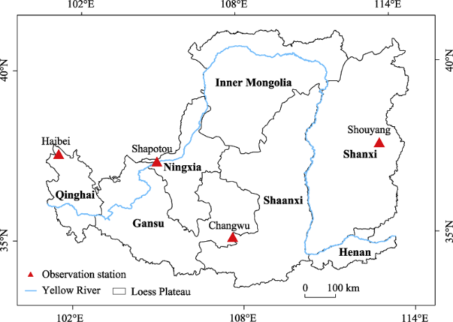
Figure 1 Location of the Loess Plateau and the four observation stations for validation
Owing to the poor viscosity and friability of loess, the LP is easily eroded by running water, forming a fragmented surface morphology dominated by yuan (large flat surface with little or no erosion), ridges, hills and gullies. This region is dominated by a temperate continental climate with an average annual precipitation of approximately 466 mm, ranging from 120 mm in the northwest to 700 mm in the southeast in a substantially evaporative year. Approximately 60% of precipitation is concentrated from June to September in the form of high-intensity rainstorms (Zhao et al., 2013). The range of mean annual temperature from northwest to southeast is 4.3-14.3℃ (Guo et al., 2010).
Extensive human activities have caused serious damage to vegetation on the LP. Unreasonable land reclamation and utilization is an important factor that exacerbates soil erosion. All these factors make LP one of the most serious soil and water erosion areas in the world (Li et al., 2015).

2.2 Data collection

Meteorological data (from 2000-2015), mainly including daily precipitation, air temperature, air pressure, relative humidity, wind speed and sunshine duration, were obtained from the China Meteorological Data Service Centre (http://data.cma.cn/) at 65 stations located on and around the LP. All meteorological data were spatially interpolated to raster maps by gradient inverse distance square (GIDS) method.
The leaf area index (LAI) and albedo (α) datasets, including the black-sky albedo and the white-sky albedo, were collected from the Global Land Surface Satellite (GLASS) (http://glass-product.bnu.edu.cn/) with a temporal resolution of 8 days and a spatial resolution of 0.05°.
The solar zenith angle (SZA) data were derived from global surface reflectance datasets from the AVHRR Long Term Data Record (LTDR) (https://www.ncdc.noaa.gov/cdr/terrestrial/avhrr-surface-reflectance) with an interval of 1 day and a spatial resolution of 0.05°. We averaged daily SZA to obtain 8-day data.
The land cover data were obtained from the “Land Cover Atlas of the People's Republic of China (1:1000,000)”. The land cover maps with a resolution of 30 m covered 2000, 2005 and 2010, which represented three five-year periods (2000-2005, 2006-2010, and 2011-2015, respectively). The spatial resolution of all the datasets was resampled to 1 km.
The validation data include data from two flux tower sites (Haibei and Shouyang), two on-site measurements (Changwu and Shapotou) and the ETWatch product. Flux tower data were obtained from the Chinese terrestrial ecosystem flux observation and research network (ChinaFLUX). On-site measurements (from 2004 to 2009) were provided by the National Earth System Science Data Center (http://www.cnern.org.cn/data/). The ETWatch dataset (from 2000 to 2015) with a spatial resolution of 1 km was derived from the Institute of Remote Sensing and Digital Earth, Chinese Academy of Sciences (CAS). This dataset was demonstrated to successfully simulate ET on a large scale with a deviation of approximately 10% in the growing season (Wu et al., 2012).

2.3 Analysis of spatiotemporal vegetation and evapotranspiration changes

The Sen + Mann-Kendall trend method was used to analyze the interannual changes in vegetation and ET. Sen slope estimation (Sen, 1968) is a robust method for identifying nonparametric statistical trends. It has a good ability to prevent outliers and measurement errors and is often used in the trend analysis of long-term series data.
The Mann-Kendall method (Mann, 1945; Kendall, 1990), as a nonparametric statistical test, does not require the measured value to obey a normal distribution, nor does it require the trend to be linear, and it is not affected by missing values or outliers. Therefore, Sen + Mann-Kendall trend analysis has become an important method for evaluating time series trends and has been widely used in the analysis of vegetation time series changes (De Beurs et al., 2005).
The Sen slope estimation is calculated with the following equation:
$\beta =mean\left( \frac{{{\text{x}}_{\text{j}}}-{{\text{x}}_{\text{i}}}}{\text{j}-\text{i}} \right),\forall \text{j}>\text{i}$
where xj and xi are the j-th and i-th time series data, respectively; β > 0 indicates an upward trend; and β < 0 indicates a downward trend.
The Mann-Kendall test statistic is calculated as follows:
$S=\sum\limits_{\text{i}=1}^{n-1}{\sum\limits_{j=i+1}^{n}{sign\left( {{\text{x}}_{\text{j}}}-{{\text{x}}_{\text{i}}} \right)}}$
$sign\left( \theta \right)=\left\{ \begin{matrix} 1 & {} & \left( \theta >0 \right) \\ 0 & {} & \left( \theta =0 \right) \\ -1 & {} & \left( \theta <0 \right) \\\end{matrix} \right.$
where S is the test statistic, xj and xi are the time series data, and n is the number of samples in the series. When n ≥ 10, the statistic S approximately obeys the standard normal distribution, and the standardized test statistic Z is calculated using the following formulas:
$Z=\left\{ \begin{matrix} \frac{S}{\sqrt{V\text{ar}\left( S \right)}} & {} & \left( S>0 \right) \\ 0 & {} & \left( S=0 \right) \\ \frac{S+1}{\sqrt{V\text{ar}\left( S \right)}} & {} & \left( S<0 \right) \\\end{matrix} \right.$
$V\text{ar}\left( S \right)=\frac{\text{n}\left( \text{n}-1 \right)\left( 2\text{n}+5 \right)}{18}$
Under the given significance level α, taken here as 0.05, $\left| Z \right|>{{Z}_{1\text{-}\alpha /2}}$ indicates that the time series data have passed the test, that is, there is an obvious trend change. Otherwise, the null hypothesis that the trend is not significant is accepted.

2.4 Simulation of evapotranspiration

ET represents the sum of all the processes in which water enters the atmosphere from the land surface and is composed of three parts: vegetation transpiration (Ec), soil evaporation (Es) and canopy interception evaporation (Ei). When the underlying surface has a sufficient water supply, the ET is approximately equal to the potential ET, but the underlying surface is always inadequately supplied under natural conditions. The amount of water that actually enters the atmosphere from the underlying surface is called actual ET.
We developed a simplified remote sensing-based ET model that combined the PM and PT-JPL methods. Among them, the PM formula is, in theory, a more accurate method for calculating the potential ET than the PT formula. It is generally believed that the PM formula fully considers various factors affecting ET and has high accuracy and wide applicability in both arid and humid regions (Allen et al., 1998). Therefore, it is a standard formula for calculating potential ET. Then, we used a series of limiting factors based on meteorology and plant physiology and ecology to convert potential ET into actual ET, referring to the PT-JPL model developed by Fisher et al. (2008).
$ET={{E}_{c}}+{{E}_{s}}+{{E}_{i}}$
Actual vegetation transpiration (Ec) is estimated based on potential transpiration, restricted by the minimum stomatal resistance of a specific vegetation type and environmental pressures such as temperature and moisture. The potential transpiration is defined as the potential transpiration rate (Ecp).
${{E}_{\text{c}}}=\left( 1-{{\text{f}}_{\text{wet}}} \right){{E}_{\text{cp}}}{{\text{f}}_{\text{t}}}{{\text{f}}_{\text{w}}}$
${{\text{f}}_{\text{wet}}}=R{{H}^{4}}$
${{E}_{\text{cp}}}=\frac{\Delta {{R}_{\text{nc}}}+{{\text{f}}_{\text{c}}}\rho {{C}_{\text{p}}}D/{{\text{r}}_{\text{a}}}}{\lambda \left( \Delta +\gamma \eta \right)}$
where fwet is the relative surface wetness; Ecp is the potential transpiration rate (mm d‒1); ft is the plant temperature constraint; fw is the plant moisture constraint; RH is the relative humidity (%); λ is the latent heat of vaporization of water (J kg‒1); Δ is the slope of the curve relating saturation water vapor pressure to temperature (kPa℃‒1); Rnc is the net radiation absorbed by the canopy (MJ m‒2 d‒1); fc is the fractional total vegetation cover; ρ is the air density (kg m‒3); Cp is the specific heat capacity of air (MJ kg‒1‒1); D is the saturated water vapor pressure deficit of air (kPa); ra is the aerodynamic resistance between the canopy and the reference height (s m‒1); γ is the psychrometric constant (kPa℃‒1); and η is the ratio of the minimum stomatal resistance of a natural plant functional type to that of the reference crop according to the minimum resistances adopted in previous studies (Leuning et al., 2008; Bastiaanssen et al., 2012).
When the air is in a regular state of advection, ra for short grassland is calculated as
${{\text{r}}_{\text{a}}}=\frac{{{\ln }^{2}}\left[ \left( \text{z}-\text{d} \right)/{{z}_{\text{o}}} \right]}{{{\text{k}}^{2}}{{\text{u}}_{\text{a}}}}=208/{{\text{u}}_{\text{a}}}$
where z is the reference height; d is the zero plane displacement; zo is the roughness length; k is the von Karman constant, 0.41; and ua is the wind velocity (m s‒1).
The transmittance of light through the canopy can be used to measure fc considering the vegetation elements as opaque. When light passes down through the top of the canopy, the light transmittance (Ptr) can be simulated using an exponential model (Xiao et al., 2016):
${{\text{f}}_{\text{c}}}=1-{{P}_{\text{tr}}}\left( 0 \right)$
${{P}_{\text{tr}}}\left( \varphi \right)={{\text{e}}^{-\sqrt{\text{a}}}}\times {{\text{k}}_{\text{c}}}\left( \varphi \right)\times \Omega \times LAI$
${{\text{k}}_{\text{c}}}\left( \varphi \right)=\frac{\sqrt{{{\text{x}}^{2}}+{{\tan }^{2}}\left( \varphi \right)}}{\text{x}+1.774\times {{\left( \text{x}+1.182 \right)}^{-0.733}}}$
where a is the absorptivity of leaves for radiation; $\Omega $is the clumping index taking into account the nonrandom spatial distribution of phytoelements within the canopy; LAI is the leaf area index of the canopy; kc(φ) is the canopy extinction coefficient; φ is the solar zenith angle; and x is the ratio of average projected areas of canopy elements on horizontal and vertical surfaces.
The expressions of the constraint functions from air temperature (ft) and water vapor pressure deficit (fw) are as follows (Mu et al., 2007; Ke et al., 2010):
${{\text{f}}_{\text{t}}}=\exp \left. {{\left\{ -\left[ \left( {{T}_{a}}-{{T}_{opt}} \right)/{{T}_{opt}} \right] \right.}^{2}} \right\}$
${{f}_{w}}=\left( D-{{D}_{\text{o}}} \right)/\left( {{D}_{c}}-{{D}_{\text{o}}} \right)$
where Ta is the air temperature; Topt is the optimal temperature for canopy transpiration (20℃); and Do and Dc are the water vapor pressure deficits when stomata start to shrinking and close completely (set as 0.65 and 3.8 kPa), respectively.
The actual soil evaporation (Es) is constrained by the potential evaporation rate (Esp) and the soil exfiltration (Eex). Essentially, soil evaporation is a drying process in which the soil loses water. As the evaporation process continues, the water content in the soil gradually decreases, so its water supply conditions worsen, and the actual soil evaporation also decreases (Eagleson, 1978).
${{E}_{\text{s}}}=\min \left( {{E}_{\text{s}}},{{E}_{ex}} \right)$
${{E}_{\text{s}}}=\left[ {{\text{f}}_{\text{wet}}}+{{\text{f}}_{SM}}\left( 1-{{\text{f}}_{\text{wet}}} \right) \right]{{E}_{\text{sp}}}$
${{\text{f}}_{SM}}=R{{H}^{D/\beta }}$
${{E}_{\text{sp}}}=\frac{\Delta \left( {{R}_{\text{ns}}}-G \right)+\left( \text{1}-{{\text{f}}_{\text{c}}} \right)\rho {{C}_{\text{p}}}D/{{\text{r}}_{\text{as}}}}{\lambda \left( \Delta +\gamma \right)}$
where fSM is the soil moisture constraint; β (set as 1.0 kPa) defines the relative sensitivity of fSM to D; Esp is the potential evaporation rate (mm d‒1); Rns is the net radiation absorbed by the soil surface (MJ m‒2 d‒1); ras is the aerodynamic resistance between the reference height and the soil surface; and G is the soil heat flux (MJ m‒2 d‒1).
The decreasing soil moisture exfiltration rate (Eex) (mm d‒1) with the depletion of surface soil moisture is given as follows (Choudhury et al., 1998):
${{E}_{ex}}=S({{t}^{0.5}}-{{(t-1)}^{0.5}})$
where S is the soil-controlled exfiltration volume, which is determined by the soil texture and structure and is usually in the range of 3-5 mm d‒1.5, and it is set to a value of 4 mm d‒1.5 in this study; and t is the number of days that elapsed since the day following rainfall.
Canopy interception evaporation (Ei) refers to the evaporation of canopy-intercepted precipitation, which is equal to the potential evaporation on the surface of the wet canopy. Ei is calculated with the PT equation (Priestley et al., 1972) as follows:
${{E}_{i}}={{f}_{wet}}{{\alpha }_{PT}}\frac{\Delta }{\Delta +\gamma }{{R}_{nc}}$
where αPT is the Priestley-Taylor model coefficient for a wet surface condition (1.26).
The net radiation fluxes absorbed (Rn) are divided by fc into Rnc and Rns:
${{R}_{nc}}={{f}_{c}}{{R}_{n}}$
${{R}_{n\text{s}}}=\left( 1-{{f}_{\text{c}}} \right){{R}_{n}}$
The formula for net radiation (Rn) (Allen et al., 1998) is as follows:
${{R}_{n}}={{R}_{S}}-{{R}_{L}}$
${{R}_{S}}=\left( 1-\alpha \right){{R}_{\text{solar}}}$
${{R}_{\text{solar}}}=\left( {{\text{a}}_{\text{s}}}+{{\text{b}}_{\text{s}}}\frac{n}{N} \right){{R}_{o}}$
${{R}_{L}}=\left( 0.1+0.9\frac{n}{N} \right)\left( 0.34-0.14\sqrt{{{e}_{a}}} \right)\sigma {{\left( {{T}_{a}}+273 \right)}^{4}}$
where RS and RL are the incoming net shortwave radiation and the outgoing net longwave radiation (MJ m‒2 d‒1), respectively; Rsolar is solar radiation (MJ m‒2 d‒1); as and bs are the regression coefficients, and we used the radiation observation data of Wang et al. (2012b) to calculate the average radiation coefficients (as = 0.186, bs = 0.556) of 10 observation stations near the study area; α is the land surface albedo; n and N are the actual and potential sunshine durations (h d‒1), respectively; Ro is the solar radiation at the top of the atmosphere (MJ m‒2 d‒1); ea is the air vapor pressure (kPa); and σ is the Stefan-Boltzmann constant.
The actual albedo (α) can be calculated by combining the black-sky albedo (αdir) and the white-sky albedo (αdif):
$\alpha ={{f}_{dir}}{{\alpha }_{dir}}+{{f}_{dif}}{{\alpha }_{dif}}$
${{f}_{dir}}+{{f}_{dif}}=1.0$
${{f}_{dif}}=a{{\left( \cos \varphi \right)}^{b}}$
where fdir and fdif are the ratios of direct light and diffuse light to the total incoming light, respectively, and a and b are the regression coefficients (set as 0.123 and -0.842, respectively).

2.5 Estimation of cooling and humidifying effect

In this study, the cooling and humidifying effect means that vegetation consumes water and vaporizes it through ET during the growing season (from June to September), thereby increasing air humidity and reducing the temperature by absorbing heat. We regard the study area as a relatively closed space that does not exchange energy with the outside world. The space covers the entire LP horizontally, and the vertical height is the height of the mixed layer on the LP (677 m) (Guo, 2015).
Absolute humidity refers to the mass of water vapor per unit volume of air at a certain temperature. The total flux of water vapor transported by vegetation and the ground as a whole to the atmosphere is the actual ET. Therefore, the daily absolute humidity change (Δa) in the study area through ET is as follows (Yang, 1994; Xiao et al., 2019):
$\Delta \text{a}=\left( {{Q}_{\text{wd}}}\times 1000 \right)\text{/}V$
$V=S\times \text{h}$
where Δa is the daily increase in absolute humidity (g m‒3 d‒1); Qwd is the actual daily ET (kg d‒1); V is the air volume within the height of the mixed layer in the study area (m3); S is the total area (m2); and h is the height of the mixed layer (m).
Thus, the daily increment of water vapor pressure (Δe) (hPa d‒1) in the study area is
$\Delta \text{e}=\left( \Delta \text{a}\times T \right)\text{/}218$
where T is the absolute temperature (K).
Then, the saturated vapor pressure (es) is calculated using the following formula:
${{\text{e}}_{\text{s}}}=\exp \left[ 21.382-\left( \frac{5.3475\times {{10}^{3}}}{T} \right) \right]$
Therefore, the daily increment in relative humidity (Δf) in the study area is estimated as
$\Delta \text{f}=\frac{\Delta \text{e}}{{{\text{e}}_{\text{s}}}}\times 100%$
The ET process is accompanied by energy consumption and conversion of latent and heat energy. Since the latent heat of vaporization refers to the heat required for a substance to transform from the liquid phase to the gas phase at a constant temperature, the latent heat of vaporization of water can be used to calculate the heat absorption of ET. The calculation formula of latent heat of evaporation (L) is
$L=\left( 597-\frac{5}{9}T \right)\times 4.1859$
where L is the heat absorbed per kilogram of water vaporized (kJ kg‒1) when the temperature is T (℃).
The heat absorption in the study area during the growing season is
${{Q}_{\text{h}}}=\sum {{Q}_{\text{wi}}}\times L\times {{S}_{\text{i}}}$
where Qh is the heat absorption (kJ); Qwi is the ET of the i-th grid; and Si is the grid area (1 km2).
Since ET consumes energy in the surrounding air and thus reduces the temperature, the daily cooling effect in the study area is as follows:
$\Delta T={{Q}_{\text{hd}}}\text{/}\left( V\times {{\rho }_{\text{c}}} \right)$
where ΔT is the daily temperature reduction (℃ d‒1); Qhd is the daily heat absorption (kJ d‒1); and ρc is the volumetric heat capacity of air, with a value of 1.256 kJ m‒3 ‒1.

3 Results and analysis

3.1 Changes in vegetation spatiotemporal pattern

According to results of Sen trend analysis and Mann-Kendall test, vegetation restoration was divided into five categories. β > 0 and |Z| > 1.96 indicated a significant improvement in vegetation coverage, β > 0 and |Z| < 1.96 indicated a nonsignificant improvement, β = 0 indicated basically unchanged coverage, β < 0 and |Z| < 1.96 indicated nonsignificant degradation, and β < 0 and |Z| > 1.96 indicated significant degradation of vegetation.
The vegetation cover generally showed an upward trend, and only a few parts of the LP were degraded. Vegetation coverage increased in 91.87% of the area, 3.51% of the area remained basically unchanged, 3.82% was slightly degraded, and only 0.80% had obvious vegetation degradation (Table 1). In general, the restoration of vegetation in Shanxi and Shaanxi provinces was the most obvious. The ecological environment of Gansu and Henan Provinces had also been improved. Inner Mongolia, Qinghai and Ningxia had relatively slow vegetation restoration, and ecological construction should be further strengthened.
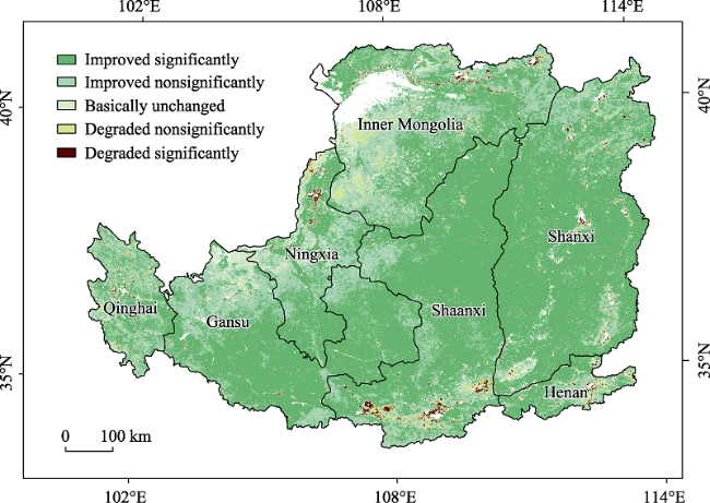
Table 1 The effect of vegetation restoration on the Loess Plateau
Regions Improved
significantly (%)
Improved
nonsignificantly (%)
Basically
unchanged (%)
Degraded
nonsignificantly (%)
Degraded
significantly (%)
Inner Mongolia 46.13 38.28 8.79 5.94 0.87
Gansu 68.19 26.46 4.03 1.19 0.13
Shanxi 79.93 16.38 0.47 2.68 0.54
Qinghai 42.88 44.63 3.50 8.10 0.90
Shaanxi 75.81 18.53 0.51 3.86 1.29
Ningxia 52.01 34.59 9.11 3.23 1.06
Henan 53.08 33.52 0.76 10.24 2.40
65.67 26.20 3.51 3.82 0.80
Although the LAI during the growing season on the LP showed a significant growth trend overall, there were obvious spatial differences among regions. The vegetation restoration on the southeastern LP was significantly better than that on the northwestern LP (Figure 2). Due to the scarce water resources, severe desertification and poor growing conditions for vegetation, the vegetation coverage was relatively poor in the northwest compared with that in the southeast. However, with the development of the Grain for Green Project, the vegetation coverage on the LP has been significantly improved. The vegetation has been obviously restored, and the ecological environment has been substantially improved in various regions, including the Mu Us Sandy Land from Ordos to Yulin, Ziwuling and Huanglong Mountain forests in Yan'an, the Lvliang-Taihang mountainous area in Shanxi, the mountainous areas of western Henan, eastern and central Gansu, and southeastern Ningxia. This result was closely related to the nationwide ecological restoration project since 1999. Significantly degraded areas were mainly concentrated in provincial capitals or central cities such as the Guanzhong city agglomeration, Luoyang, Taiyuan, Datong, Yinchuan, Baotou, and Xining. In these regions, due to rapid economic development and urbanization, the rapid expansion of urban land has led to the rapid degradation of vegetation. This result was consistent with previous studies (Zheng et al., 2019; Li et al., 2020; Shao et al., 2021).
Figure 2 Changes in the growing season LAI on the Loess Plateau

3.2 Validation of the estimated evapotranspiration

To validate the estimated monthly ET, we compared the estimated ET with the collected ET observation data from two flux tower sites (Haibei and Shouyang) and two on-site measurements (Shapotou and Changwu) on the LP. The results showed good consistency, with RMSEs ranging from 11.98 mm month‒1 (Haibei) to 24.52 mm month‒1 (Changwu), corresponding R2 values ranging from 0.60 to 0.93, and bias values ranging from -10.50 to 5.06 mm (Figures 3 and 4). The ETWatch results at the monthly scale were also used to validate the estimated ET from 2000 to 2015 (Figure 5). The results showed that the two fluctuated synchronously and had a strong correlation in long-term changes (R2 = 0.62, RMSE = 20.52, bias = -3.61).
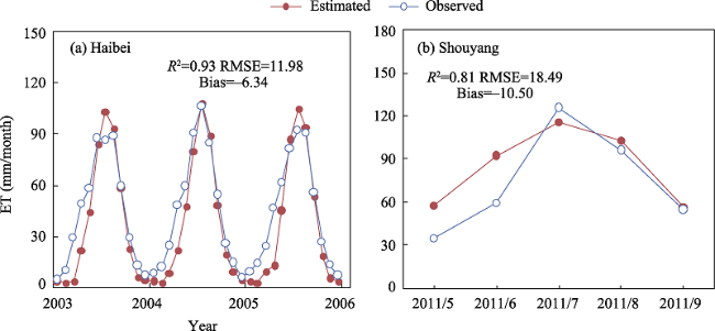
Figure 3 Monthly time-series comparisons between estimated and observed ET from flux tower sites
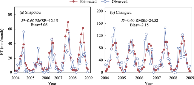
Figure 4 Monthly time-series comparisons between estimated and observed ET from two on-site measurements
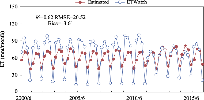
Figure 5 Monthly time-series comparisons between estimated ET and ET dataset from ETWatch model
Compared with the observed data, the estimated ET was slightly underestimated. This may be caused by the failure to consider the impact of the massive construction of silt dams on the LP in the 1970s. Most silt dams were small in size and cannot be identified by sensors. However, as time passes, the dams were gradually filled with eroded materials, with increasingly weaker influences on the hydrological process. Therefore, this limitation did not have a significant impact on the final result (Xu et al., 2004; Wang et al., 2015).
Finally, we used the Nash-Sutcliffe efficiency coefficient (NSE) (Legates et al., 1999) to evaluate the performance of the model based on all the validation data. The good performance (NSE = 0.72) indicated that the method can be used to estimate ET of the LP.

3.3 Spatial and temporal variation in evapotranspiration

In general, the actual ET during the growing season on the LP had a strong correlation with LAI (R = 0.753, p < 0.001), and the interannual changes also showed good consistency. The actual ET and LAI minimums appeared in 2001 and were 227.652 mm and 0.940, respectively, and the maximums appeared in 2014 (271.770 mm) and 2013 (1.605). The LAI increased significantly at an annual rate of 0.0364 (p < 0.001), and the actual ET also showed a significant increasing trend (p < 0.05), with an average annual increase of 1.6251 mm (Figure 6).
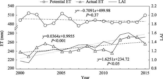
Figure 6 Interannual trend of ET in the growing season on the Loess Plateau
The spatial distributions of actual ET and LAI both presented prominent geographical heterogeneity. Approximately 51.73% of the study area showed an upward trend in the actual ET, and the area with a significant increase accounted for 9.61% (p < 0.05). The highest trend appeared from the northeast to southeast of the LP (Figure 7). The greening trend of LAI was overwhelming (91.87%), and the most significant greening trend was also distributed in the area between the northeast and southeast of the LP (Figure 2).
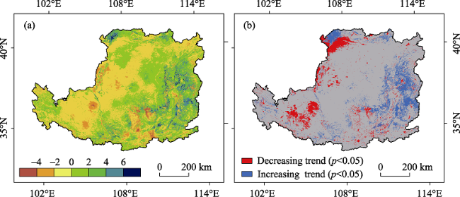
Figure 7 Spatial distributions of (a) trend and (b) significance of actual ET in the growing season on the Loess Plateau
In contrast, the potential ET decreased by an approximate rate of 0.7091 mm yr‒1 (p = 0.37). The potential ET minimums that appeared in 2003 and 2007 were 475.87 mm and 473.69 mm, respectively (Figure 6). The annual potential ET decreased over large areas in the LP (77.55%), with the sharpest decrease in the southwestern parts of the LP (Figure 8). The potential ET showed a downward trend, which was consistent with the trend of observed or pan evaporation in many regions (Cong et al., 2008). The reduction was mainly caused by the decrease in wind speed, which was usually considered to be related to weak atmospheric circulation and increased surface roughness caused by the Grain for Green Project. In addition, the reduction in solar radiation was also one of the reasons for the reduction in potential ET (Yin et al., 2010; Shi et al., 2017).
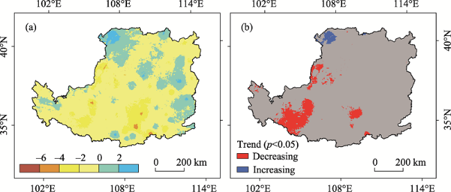
Figure 8 Spatial distributions of (a) trend and (b) significance of potential ET in the growing season on the Loess Plateau

3.4 Cooling and humidifying effect

The daily absolute humidity from June to September in 2000 to 2015 increased by 2.76-3.29 g m‒3, with the smallest increase in 2001 and the greatest in 2014 (Table 2), and the relative humidity increased by 15.43%-19.31%. Similarly, for both absolute humidity and relative humidity, the lowest and highest values appeared in 2001 and 2014, respectively (Table 3).
Table 2 Absolute humidity increment during the growing season on the Loess Plateau
Regions Absolute humidity increment (g m‒3 d‒1)
2000 2001 2002 2003 2004 2005 2006 2007 2008 2009 2010 2011 2012 2013 2014 2015
Inner Mongolia 1.76 1.67 2.02 2.19 2.11 1.73 1.86 1.94 2.09 1.90 1.94 1.77 2.31 2.43 2.29 1.87
Gansu 2.67 2.68 2.67 2.90 2.76 2.78 2.68 2.79 2.92 2.72 2.82 2.67 3.04 3.19 3.20 3.05
Shanxi 3.65 3.34 3.71 3.74 3.70 3.65 3.61 3.56 3.70 3.58 3.59 3.63 3.80 3.87 3.91 3.81
Qinghai 3.17 3.26 3.12 3.30 3.18 3.25 3.24 3.23 3.26 3.18 3.36 3.16 3.24 3.24 3.22 3.11
Shaanxi 3.27 3.15 3.51 3.54 3.44 3.35 3.32 3.39 3.49 3.36 3.30 3.27 3.69 3.66 3.75 3.64
Ningxia 1.98 1.94 2.14 2.25 2.20 1.81 1.91 2.04 1.97 2.06 2.27 2.02 2.43 2.62 2.66 2.24
Henan 4.11 3.88 3.89 4.06 4.20 3.86 3.85 3.81 3.85 3.71 3.56 3.13 3.79 3.64 3.79 4.01
2.88 2.76 3.00 3.11 3.04 2.89 2.89 2.94 3.04 2.91 2.95 2.85 3.21 3.28 3.29 3.10
Table 3 Relative humidity increment during the growing season on the Loess Plateau
Regions Relative humidity increment (% d‒1)
2000 2001 2002 2003 2004 2005 2006 2007 2008 2009 2010 2011 2012 2013 2014 2015
Inner Mongolia 9.60 8.96 11.23 12.56 12.46 9.08 10.18 10.83 11.91 10.49 10.24 9.56 13.32 13.40 13.33 10.78
Gansu 16.46 16.58 16.29 18.42 17.66 16.89 15.94 17.75 18.48 16.77 17.06 16.13 18.93 19.40 20.67 19.62
Shanxi 19.86 17.80 20.29 21.21 21.42 19.08 19.49 19.54 20.70 19.34 18.99 19.33 21.51 20.72 22.00 21.02
Qinghai 24.88 25.47 24.20 26.39 25.87 25.04 24.45 25.82 26.09 24.82 24.91 23.51 25.26 24.43 25.63 24.65
Shaanxi 17.27 16.43 18.36 19.22 18.90 17.11 17.21 18.40 18.97 17.86 17.01 16.85 20.04 18.85 20.40 19.59
Ningxia 11.53 11.27 12.52 13.39 13.39 10.13 10.78 12.16 11.63 11.96 12.90 11.18 14.12 14.91 15.79 13.12
Henan 18.80 17.17 17.06 19.36 19.85 17.21 17.23 17.82 17.85 16.83 16.17 13.66 17.14 15.29 18.25 19.44
16.27 15.43 16.89 18.20 18.02 15.87 16.06 16.97 17.70 16.47 16.26 15.73 18.62 18.23 19.31 17.98
The absolute humidity increment was determined by the actual ET and area, and the actual ET was significantly correlated with the LAI. For different provinces, the absolute humidity increments in decreasing order were Henan, Shanxi, Shaanxi, Qinghai, Gansu, Ningxia, and Inner Mongolia, which was basically consistent with the distribution of the LAI. Among them, the average annual LAI in Shaanxi was slightly higher than that in Shanxi, but the absolute humidity increment in Shaanxi was slightly lower than that in Shanxi due to the influence of regional area. For relative humidity, the increment in Qinghai was the highest, followed by Shanxi and Shaanxi, and those in the other four provinces were lower, which may be affected by the temperature. Although the absolute humidity increment in Qinghai was relatively low, the temperature in this area was significantly lower than that in the other provinces, resulting in the maximum relative humidity increment. Similarly, although the daily absolute humidity increment in Henan was the highest, the average temperature in this area was higher, resulting in a lower daily increase in relative humidity. Because the temperatures in the other four provinces were similar, there was no significant difference in the distribution of absolute humidity and relative humidity increments.
Tables 4 and 5 show that daily heat absorption had a good synchronization with temperature change from 2000 to 2015. The heat absorption through ET on the LP from June to September was 3.47×10¹⁷ kJ yr‒1 to 4.15×10¹⁷ kJ yr‒1, and the daily cooling was 5.38- 6.43℃ d‒1. The endothermic and cooling effects were the best in 2014 (4.15×10¹⁷ kJ and 6.43℃), and the lowest values appeared in 2001 (3.47×10¹⁷ kJ and 5.38℃), respectively.
Table 4 Heat absorption during the growing season on the Loess Plateau
Regions Heat absorption (1017 kJ)
2000 2001 2002 2003 2004 2005 2006 2007 2008 2009 2010 2011 2012 2013 2014 2015
Inner Mongolia 0.44 0.41 0.50 0.54 0.52 0.43 0.46 0.48 0.52 0.47 0.48 0.44 0.57 0.60 0.57 0.44
Gansu 0.59 0.59 0.59 0.64 0.61 0.62 0.59 0.62 0.65 0.60 0.63 0.59 0.67 0.71 0.71 0.59
Shanxi 1.17 1.07 1.19 1.20 1.19 1.17 1.15 1.14 1.19 1.14 1.15 1.16 1.22 1.24 1.25 1.17
Qinghai 0.22 0.22 0.21 0.23 0.22 0.22 0.22 0.22 0.22 0.22 0.23 0.22 0.22 0.22 0.22 0.22
Shaanxi 0.86 0.83 0.93 0.93 0.91 0.89 0.88 0.90 0.92 0.89 0.87 0.86 0.97 0.97 0.99 0.86
Ningxia 0.20 0.20 0.22 0.23 0.22 0.18 0.19 0.21 0.20 0.21 0.23 0.21 0.25 0.27 0.27 0.20
Henan 0.15 0.14 0.14 0.15 0.16 0.14 0.14 0.14 0.14 0.14 0.13 0.12 0.14 0.14 0.14 0.15
3.63 3.47 3.78 3.93 3.83 3.65 3.64 3.71 3.84 3.67 3.72 3.59 4.05 4.14 4.15 3.63
Table 5 Temperature decrease during the growing season on the Loess Plateau
Regions Temperature decrease (℃ d-1)
2000 2001 2002 2003 2004 2005 2006 2007 2008 2009 2010 2011 2012 2013 2014 2015
Inner Mongolia 3.44 3.26 3.94 4.27 4.12 3.37 3.64 3.80 4.07 3.71 3.78 3.45 4.52 4.74 4.47 3.65
Gansu 5.22 5.23 5.21 5.68 5.40 5.43 5.23 5.46 5.70 5.31 5.51 5.21 5.94 6.22 6.25 5.96
Shanxi 7.11 6.51 7.24 7.30 7.23 7.11 7.04 6.94 7.23 6.98 6.99 7.07 7.41 7.55 7.63 7.44
Qinghai 6.21 6.40 6.12 6.47 6.23 6.37 6.35 6.33 6.39 6.24 6.59 6.19 6.36 6.35 6.32 6.11
Shaanxi 6.37 6.15 6.85 6.90 6.71 6.54 6.46 6.62 6.80 6.55 6.43 6.37 7.19 7.13 7.31 7.10
Ningxia 3.87 3.80 4.19 4.40 4.31 3.54 3.72 3.98 3.85 4.01 4.43 3.93 4.74 5.12 5.19 4.37
Henan 8.00 7.55 7.56 7.90 8.17 7.51 7.49 7.41 7.49 7.21 6.93 6.08 7.37 7.06 7.38 7.80
5.62 5.38 5.86 6.08 5.93 5.64 5.64 5.74 5.94 5.68 5.75 5.56 6.27 6.40 6.43 6.05
Spatially, heat absorption through the ET process was higher in Shanxi and Shaanxi and lower in Henan. In terms of the cooling effect, Henan showed the best cooling effect, while Ningxia and Inner Mongolia had relatively poor cooling effects. The amount of heat absorption was determined by the actual ET and temperature. Since the results were the total heat absorption of each province, the total ET dominated the total heat absorption on a large regional scale, although the temperature in each province was different, and the total ET was also closely related to the area.
The decrease in average daily temperature in the study area was positively correlated with heat absorption and ET and negatively correlated with regional area and temperature. The cooling effect was consistent with the average ET in each region and the distribution of the average annual LAI, and the temperature decrease was extremely significantly correlated with the absolute humidity (R = 0.999, p < 0.001). Vegetation can reduce environmental temperature by affecting land surface ET.

3.5 Vegetation restoration controls on temperature and humidity

From the above analysis, it can be seen that the LAI and ET had significant synchronization. Although the cooling and humidifying effect was generally consistent with the spatial distribution of the LAI, there were still differences in details, and they may be affected by other factors, such as temperature. It was generally believed that LAI was positively correlated with canopy transpiration, negatively correlated with soil evaporation, and positively correlated with total ET (Forrester et al., 2012; Sun et al., 2014). However, it was also been found that LAI was obviously negatively correlated with ET (Limpens et al., 2014).
Therefore, the correlation between LAI and actual ET, cooling and humidifying based on annual and monthly scales was determined to further study the contribution of vegetation restoration to the cooling and humidifying effect.
The results (Tables 6 and 7) showed that LAI was significantly positively correlated with actual ET, cooling and humidification on annual and monthly scales (p < 0.01). The influence of vegetation on relative humidity was lower than its influence on other indicators (R = 0.511, 0.720). Because the daily increase in water vapor pressure and saturated water vapor pressure were affected by temperature (T), partial correlation analysis with T as the control variable was used to more deeply analyze the impact of vegetation cover changes on climate. The results showed that the correlation between LAI and relative humidity and the correlation between actual ET and relative humidity were significantly improved (p < 0.01), which indicated that relative humidity was affected by both vegetation and environmental factors. From the perspective of correlation coefficients, the monthly and annual scale analysis results were consistent, and the analysis results at the monthly scale were better than those at the annual scale.
Table 6 Correlation analysis on the annual scale
Actual ET Absolute humidity Relative humidity Heat absorption Temperature decrease
RLAI 0.753 0.753 0.511 0.751 0.751
RET 1 1.000 0.887 1.000 1.000
RLAI·T 0.795 0.795 0.71 0.795 0.795
RET·T 1 1 0.979 1 1

RLAI·T and RET·T refer to the partial correlation coefficients that exclude T.

Table 7 Correlation analysis on the monthly scale
Actual ET Absolute humidity Relative humidity Heat absorption Temperature decrease
RLAI 0.792 0.792 0.720 0.793 0.793
RET 1 1.000 0.661 1.000 1.000
RLAI·T 0.78 0.78 0.763 0.78 0.78
RET·T 1 1 0.992 1 1

RLAI·T and RET·T refer to the partial correlation coefficients that exclude T.

To study the relationship between ΔLAI and climate change, the relationships between the annual LAI, actual ET changes and climate factors in each province were investigated.
Figures 9 and 10 show that the changes in vegetation cover and actual ET were spatially positively correlated. The data show that vegetation cover increased and decreased with the actual ET and humidity at the same time, making up approximately 64.76% of the total data, and approximately 63.81% of the data points changed simultaneously with the vegetation cover, heat absorption, and temperature. Moreover, changes in actual ET were approximately linearly related to climate fluctuations.
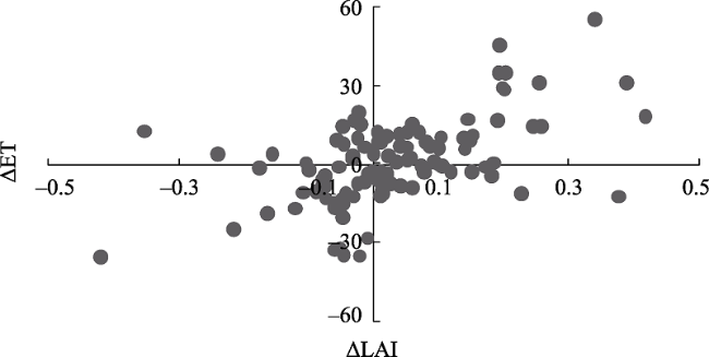
Figure 9 The relationships between the changes in ET and LAI on the Loess Plateau
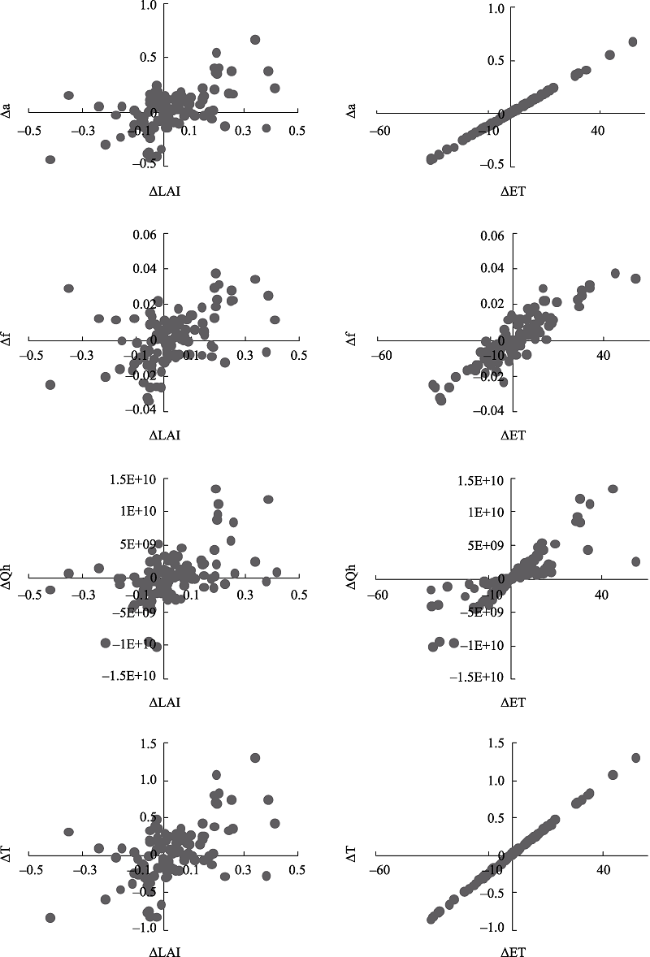
Figure 10 Relationships between the changes in cooling and humidifying and LAI or ET on the Loess Plateau
The results of space-based calibration analysis and correlation analysis were highly consistent, which further showed that vegetation can regulate the local microclimate by affecting land surface ET.

4 Discussion

4.1 Impact of vegetation on cooling and humidification

In this study, we focused on the impact of vegetation restoration on local microclimate. Vegetation trend analysis suggested that vegetation coverage in most areas of the LP has been obviously improved, as indicated by increased LAI, after more than ten years of the Grain for Green Project.
Vegetation growth changes are the consequence of climate change and human activities. Some studies from process models suggested that China's afforestation activity could better explain the spatial patterns of the trend in vegetation growth (Piao et al., 2015). This is particularly true on the LP. The analysis of a variety of MODIS products showed that the Grain for Green Project has significantly increased the tree cover of the LP (Xiao et al., 2014). A similar conclusion was also corroborated by many previous studies (Zhang et al., 2011a; Li et al., 2017). Ecological conservation policies such as the Grain for Green Project in this area was the primary reason for the increase in overall vegetation growth (vegetation greening) and ET on the LP (Liang et al., 2020).
The LAI, closely related to the growth status of plant, is an important indicator reflecting the leaf area and canopy structure of plants (Lin et al., 2003). LAI has been widely used to describe vegetation changes and it is believed to be able to describe the dynamic changes in vegetation more robustly than the NDVI (Xiao et al., 2014). Therefore, the influence of LAI on ET could generally represent the effect of vegetation restoration, which is consistent with previous results (Bréda et al., 1996; Zhang et al., 2015).
We found that vegetation restoration had a significant impact on the temperature and humidity on the LP. The better the vegetation coverage is, the better the overall cooling and humidifying effect. The average LAI in the growing season from 2000 to 2015 increased by 0.0364 per year (p < 0.05), increasing the daily absolute humidity by 2.76-3.29 g m‒3 and the relative humidity by 15.43%-19.31%. The annual heat absorption was estimated to be 3.47-4.15×10¹⁷ kJ yr‒1, and the daily temperature decrease ranged from 5.38 to 6.43℃. Liang et al. (2006) used the new nonhydrostatic atmospheric mesoscale model MM5 of the National Center for Atmospheric Research (NCAR) to compare and analyze the changes in various meteorological elements in the vegetation change area by changing the vegetation coverage in local areas of the LP. The results indicated that improved vegetation can increase precipitation and moisture and reduce runoff and diurnal changes in air temperature. Zhang et al. (2013) compared plant communities with bare land and found that small plant communities can lead to a decrease in temperature and an increase in relative humidity through field measurements, and the temperature reduction and relative humidity increase were larger in summer than in other seasons. Jin et al. (2020) investigated the impact of surface vegetation changes on the surface temperature of the LP based on the observation minus reanalysis (OMR) method. It was found that the restoration of vegetation on the LP reduced the temperature by 0.02 ℃ every ten years from 1982 to 2015. The results of this study are comparable to those of other studies, and vegetation has a significant cooling and humidifying effect during the growing season.
The scale of changes in climate factors was different, and we found that the impact of vegetation on microclimate was more significant on the monthly scale. There are time lags in the response of the vegetation to climate factors. Many studies have been conducted on the response characteristics of vegetation to climate in different regions. In China, vegetation is always closely related to water and heat factors such as precipitation and temperature, and the lag time of the precipitation response is generally longer than that of the temperature response (Cui et al., 2009; Rammig et al., 2014; Kong et al., 2020). The analysis of the correlation between the vegetation (LAI) and temperature (T) (Table 8) indicated that there was no significant correlation between vegetation and temperature on the growing season scale (R = -0.113, p = 0.677), which showed that the relationship between the interannual variation in vegetation and the temperature in the growing season was not close. However, the relationship between vegetation changes and temperature cannot be fully explained by only the interannual changes due to the scale difference of changes in climate factors. Nevertheless, these changes in vegetation coverage and temperature were significantly correlated on a monthly scale. The LAI of the growing season had the strongest correlation with the temperature of the current month (R = 0.540, p < 0.001). The response of vegetation to temperature had no obvious time lag on the monthly scale.
Table 8 Correlation analysis between LAI and temperature (T)
LAI and T Growing season Current month Last month The month before last
R ‒0.113 0.540 0.336 0.009
p 0.677 0.000 0.007 0.945

4.2 Interaction between vegetation and climate

There are complex interactions between vegetation and climate. Vegetation can regulate the climate, and climate change can also profoundly affect vegetation growth, especially in ecologically fragile areas such as the LP, because vegetation is constantly adapting to changes in the climate and environment. Temperature is the controlling factor of vegetation change in the growing season. Both high temperature and low temperature inhibit the growth of vegetation, and suitable temperature can promote the growth of vegetation. Some studies found that an increase in temperature results in a negative impact when the average temperature during the growing season is lower than 11℃ because the increase in temperature makes the soil dry in summer, which is not conducive to vegetation growth (Oki et al., 2006). Precipitation is an important constraining factor for vegetation growth, and precipitation is significantly related to vegetation coverage. Soil water stress can cause physiological metabolic disorders in crop plants and consequently reduce photosynthetic performance, leaf area, chloroplast content, and population photosynthetic performance (Jiang et al., 2007).
In different climatic regions and ecosystems, the factors that control ET are quite different, but the regulation of vegetation plays an important role in all scenarios (Wang et al., 2012a). The interannual variation in vegetation physiological activities dominates the interannual variation in ET during the vegetation growing season, and the vegetation index is closely related to ET. Vegetation can affect surface water and heat exchange through various physiological and ecological functions and then affect the ET of the ecosystem (Baldocchi et al., 2004; Ma et al., 2019).
Transpiration and photosynthetic rates are the most important physiological characteristics of vegetation. Stomata are the main channel through which higher plants exchange water vapor and CO2 with the atmosphere, and the minimum stomatal resistance is an important parameter that determines the transpiration rate (Mo et al., 2004). In nature, various environmental factors, such as air vapor depletion, soil moisture depletion, and canopy temperature, will adjust leaf stomatal resistance. Both nonoptimal temperature and steam pressure will increase stomatal resistance (Mo, 1997). High temperature and low air humidity will increase atmospheric evaporation demand, accelerate vegetation transpiration and loss of water, and even cause stomata to close. Moreover, vegetation is very sensitive to the soil moisture. In various ecosystems, environmental factors affect ET through the physiological and ecological responses of vegetation (Yang, 2016). Therefore, we described the physiological and ecological limitations based on the coupling effect of photosynthesis and transpiration and used the limiting effects of temperature and water stress on energy absorption to characterize the limitation of the photosynthesis rate and, in turn, the transpiration rate.
Zhang et al. (2011a) simulated actual ET in typical watersheds of the LP through the SEBAL model, and the bias of daily ET was 0.51 mm. Zhang et al. (2011b) calculated the actual ET in the upper reaches of the Jinghe River Basin based on the PT and Ritchie methods, ignoring the stress effects of climate factors on vegetation, and the NSEs of the model were 0.51 and 0.55. Yang (2016) used eight major international ET models to evaluate ET on the LP, and the results showed that the best model was the PT-JPL model, which fully considered the impact of environmental factors on the physiological state of vegetation. However, other models, such as the CLM model, yielded large uncertainties in simulated ET due to insufficient parameterization of vegetation physiological processes.
Vegetation coverage determines the distribution of solar radiant energy between soil and plants, and vegetation status can also reflect that the transpiration capacity of plants is affected by environmental pressure. We obtained more accurate results because we considered the interaction between vegetation and climate and the regulatory effect of vegetation on ET.

4.3 Limitations

The increase in vegetation coverage reinforces transpiration and promotes the conversion of solar radiation to latent heat. However, at the same time, it also weakens the evaporation of soil moisture and reduces the latent heat of conversion. These processes occur simultaneously, and their interactions greatly change the energy balance of the Earth's surface, which affects the temperature. In areas with different vegetation coverage types and climatic conditions, the comprehensive effects of each process are quite different, and they will eventually play a role in increasing or decreasing temperature. The increase in the LAI is conducive to converting energy into latent heat rather than sensible heat (Yu et al., 2020a). Studies have shown that vegetation restoration can slow warming in semiarid and semihumid areas of the LP, but in arid areas with limited water, the effect of increased vegetation transpiration can only offset the impact of reduced soil water evaporation. Therefore, the increased solar radiation will not be converted into latent heat. Instead, it releases energy through sensible heat, which causes the local temperature to increase (Jeong et al., 2011; Hesslerová et al., 2019).
We analyzed the regulatory effect of the overall vegetation restoration on the local microclimate on the LP, ignoring the differences in climate change within provinces, which may slightly reduce the correlation coefficient of vegetation cooling and humidifying effects. We focused on the overall vegetation change and investigated the climate regulation effect of vegetation through ET. In fact, the cooling and humidifying effect of vegetation is affected by multiple factors, such as vegetation type, canopy closure, canopy structure, and tree height (Qin et al., 2014). More influencing factors should be considered, and more parameters need to be introduced. For instance, when estimating the potential transpiration of natural vegetation types, we ignored the difference in aerodynamic resistance among vegetation types, which may lead to insignificant deviations in estimated ET. Moreover, some highly water-consuming species disrupt the balance of water supply and demand, resulting in excessive consumption of soil water resources and leading to dry soil layers and new ecological problems (Zhang et al., 2018). Therefore, rational selection of vegetation types and design of planting density are essential for improving the ecological environment of the LP, which requires further exploration in the future.

5 Conclusions

We estimated ET on the LP and quantitatively measured the regulatory effect of vegetation restoration on the local microclimate using vegetation data, meteorological data and land cover data from 2000 to 2015. The conclusions are as follows:
(1) The LAI and actual ET on the LP both increased significantly from 2000-2015 and were strongly correlated (R = 0.753, p < 0.001).
(2) Vegetation regulated the local microclimate through ET, which increased the absolute humidity from June to September by 2.76-3.29 g m‒3 and the relative humidity by 15.43%-19.31% and decreased the temperature by 5.38-6.43°C d‒1.
(3) The cooling and humidifying effects of vegetation were also affected by the temperature in the study area, among which the change in relative humidity was most affected by temperature. The response of vegetation to temperature showed a significant correlation (R = 0.540, p < 0.001) and no time lag on a monthly scale.
[1]
Allen R G, Pereira L S, Raes D et al., 1998. Crop evapotranspiration: Guidelines for computing crop water requirements. Food and Agriculture Organization of the United Nations (FAO). Rome, Italy.

[2]
Baldocchi D, Xu L, Kiang N, 2004. How plant functional-type, weather, seasonal drought, and soil physical properties alter water and energy fluxes of an oak-grass savanna and an annual grassland. Agricultural and Forest Meteorology, 123(1/2): 13-39.

DOI

[3]
Bastiaanssen W G M, Cheema M J M, Immerzeel W W et al., 2012. Surface energy balance and actual evapotranspiration of the transboundary Indus Basin estimated from satellite measurements and the ETLook model. Water Resources Research, 48(11): W11512.

[4]
Bonan G B, 2008. Forests and climate change: Forcings, feedbacks, and the climate benefits of forests. Science, 320(5882): 1444-1449.

DOI

[5]
Bréda N, Granier A, 1996. Intra- and interannual variations of transpiration, leaf area index and radial growth of a sessile oak stand (Quercus petraea). Annales des Sciences Forestières, 53(2/3): 521-536.

DOI

[6]
Choudhury B J, Digirolamo N E, 1998. A biophysical process-based estimate of global land surface evaporation using satellite and ancillary data I: Model description and comparison with observations. Journal of Hydrology, 205(3): 164-185.

DOI

[7]
Cong Z, Yang D, Ni G, 2008. Does evaporation paradox exist in China? Hydrology and Earth System Sciences, 13(4): 357-366.

DOI

[8]
Cui L, Shi J, Yang Y et al., 2009. Ten-day response of vegetation NDVI to the variations of temperature and precipitation in eastern China. Acta Geographica Sinica, 64(7): 850-860. (in Chinese)

[9]
De Beurs K M, Henebry G M, 2005. A statistical framework for the analysis of long image time series. International Journal of Remote Sensing, 26(8): 1551-1573.

DOI

[10]
Ding Y, Li Q, Dong W, 2005. A numerical simulation study of the impacts of vegetation changes on regional climate in China. Acta Meteorologica Sinica, 63(5): 613-621. (in Chinese)

[11]
Eagleson P S, 1978. Climate, soil, and vegetation: 3. A simplified model of soil moisture movement in the liquid phase. Water Resources Research, 14(5): 722-730.

DOI

[12]
Fisher J B, Tu K P, Baldocchi D D, 2008. Global estimates of the land-atmosphere water flux based on monthly AVHRR and ISLSCP-II data, validated at 16 FLUXNET sites. Remote Sensing of Environment, 112(3): 901-919.

DOI

[13]
Forrester D I, Collopy J J, Beadle C L et al., 2012. Effect of thinning, pruning and nitrogen fertiliser application on transpiration, photosynthesis and water-use efficiency in a young Eucalyptus nitens plantation. Forest Ecology and Management, 266: 286-300.

DOI

[14]
Forzieri G, Alkama R, Miralles D G et al., 2018. Satellites reveal contrasting responses of regional climate to the widespread greening of Earth. Science, 356(6343): 1180-1184.

DOI

[15]
Fu B, Hu C, Chen L et al., 2006. Evaluating change in agricultural landscape pattern between 1980 and 2000 in the Loess hilly region of Ansai County, China. Agriculture, Ecosystems & Environment, 114(2-4): 387-396.

[16]
Gao Y, Long D, 2008. Progress in models for evapotranspiration estimation using remotely sensed data. National Remote Sensing Bulletin, 12(3): 515-528. (in Chinese)

[17]
Gou J, Wang F, Jin K et al., 2018. Cooling effect induced by vegetation restoration on the Loess Plateau. Acta Ecologica Sinica, 38(11): 3970-3978. (in Chinese)

[18]
Guo R, Li F, He W et al., 2010. Spatial and temporal variability of annual precipitation during 1958-2007 in Loess Plateau, China. In: Li D, Liu Y, Chen Y. Computer and Computing Technologies in Agriculture IV. Berlin Heidelberg Germany: Springer, 551-560.

[19]
Guo Y, 2015. Study on the influence of PM2.5 from vehicle in Guanzhong Region on ambient air quality based on CALPUFF Model[D]: Xi'an: Chang'an University. (in Chinese)

[20]
Guo Y, Wang N, Chu X et al., 2019. Analyzing vegetation coverage changes and its reasons on the Loess Plateau based on Google Earth Engine. China Environmental Science, 39(11): 4804-4811. (in Chinese)

[21]
Hesslerová P, Jan P, Hanna H et al., 2019. Wetlands:Ecosystem Services, Restoration and Wise. Cham: Springer International Publishing, 63-93.

[22]
Jeong S, Ho C, Park T, 2011. Impact of vegetation feedback on the temperature and its diurnal range over the Northern Hemisphere during summer in a 2 × CO2 climate. Climate Dynamics, 37(3/4): 821-833.

DOI

[23]
Jia X, Shao M, Wei X et al., 2020a. Policy development for sustainable soil water use on China's Loess Plateau. Science Bulletin, 65(24): 2053-2056.

DOI

[24]
Jia X, Wu H, Shao M A et al., 2020b. Re-evaluation of organic carbon pool from land surface down to bedrock on China's Loess Plateau. Agriculture, Ecosystems & Environment, 293: 106842.

[25]
Jia X, Zhao C, Wang Y et al., 2020c. Traditional dry soil layer index method overestimates soil desiccation severity following conversion of cropland into forest and grassland on China's Loess Plateau. Agriculture, Ecosystems & Environment, 291: 106794.

DOI

[26]
Jiang D, Yu Z, 2007. Effects of soil water on yeild and grain quality of wheat. Journal of Nuclear Agricultural Sciences, 21(6): 641-645. (in Chinese)

[27]
Jin K, Wang F, Zong Q et al., 2020. Impact of variations in vegetation on surface air temperature change over the Chinese Loess Plateau. Science of the Total Environment, 716: 136967.

DOI

[28]
Ke Z, Kimball J S, Nemani R R et al., 2010. A continuous satellite-derived global record of land surface evapotranspiration from 1983 to 2006. Water Resources Research, 46(9): W09522.

[29]
Kendall M G, 1990. Rank correlation methods. British Journal of Psychology, 25(1): 86-91.

[30]
Kong D, Miao C, Wu J et al., 2020. Time lag of vegetation growth on the Loess Plateau in response to climate factors: Estimation, distribution, and influence. Science of the Total Environment, 744: 140726.

DOI

[31]
Legates D R, Mccabe G J, 1999. Evaluating the use of “goodness-of-fit” measures in hydrologic and hydroclimatic model validation. Water Resources Research, 35(1): 233-241.

DOI

[32]
Leuning R, Zhang Y Q, Rajaud A et al., 2008. A simple surface conductance model to estimate regional evaporation using MODIS leaf area index and the Penman-Monteith equation. Water Resources Research, 44(10): W10419.

[33]
Li J, Peng S, Zhi L, 2017. Detecting and attributing vegetation changes on China's Loess Plateau. Agricultural and Forest Meteorology, 247: 260-270.

DOI

[34]
Li T, Lv Y, Ren Y et al., 2020. Gauging the effectiveness of vegetation restoration and the influence factors in the Loess Plateau. Acta Ecologica Sinica, 40(23): 8593-8605. (in Chinese)

[35]
Li X, Jin Z, Zhang X et al., 2015. Analysis of ecosystem management of the Loess Plateau during the past 60 years and suggestions for the furture development. Journal of Earth Environment, 6(4): 248-254. (in Chinese)

[36]
Li Y, 2001. Effects of forest on water circle on the Loess Plateau. Journal of Natural Resources, 16(5): 427-432. (in Chinese)

[37]
Liang L, Lv S, Liu Y, 2006. Numerical simulation of effect of vegetation changes of Loess Plateau on environment. Plateau Meteorology, 25(4): 575-582. (in Chinese)

[38]
Liang W, Zhang W, Jin Z et al., 2020. Rapid urbanization and agricultural intensification increase regional evaporative water consumption of the Loess Plateau. Journal of Geophysical Research: Atmospheres, 125(23): e2020JD033380.

[39]
Limpens J, Holmgren M, Jacobs C M J et al., 2014. How does tree density affect water loss of peatlands? A mesocosm experiment. PLOS ONE, 9(3): e91748.

DOI

[40]
Lin Z, Xiang Y, Mo X et al., 2003. Study on the growth model of maize leaf area index in summer Chinese Journal of Eco-Agriculture, 11(4): 74-77. (in Chinese)

[41]
Ma Z, Yan N, Wu B et al., 2019. Variation in actual evapotranspiration following changes in climate and vegetation cover during an ecological restoration period (2000-2015) in the Loess Plateau, China. Science of the Total Environment, 689: 534-545.

DOI

[42]
Mann H B, 1945. Nonparametric test against trend. Econometrica, 13(3): 245-259.

DOI

[43]
Mo X, 1997. A model for the relationship between canopy surface resistance and environmental factors and its application to evapotranspiration estimation. Geographical Research, 16(2): 81-88. (in Chinese)

[44]
Mo X, Liu S, Lin Z et al., 2004. Simulating temporal and spatial variation of evapotranspiration over the Lushi basin. Journal of Hydrology, 285(1-4): 125-142.

DOI

[45]
Mu Q, Heinsch F A, Zhao M et al., 2007. Development of a global evapotranspiration algorithm based on MODIS and global meteorology data. Remote Sensing of Environment, 111(4): 519-536.

DOI

[46]
Oki T, Kanae S, 2006. Global hydrological cycles and world water resources. Science, 313(5790): 1068-1072.

DOI

[47]
Ouyang X, Li Y, and Zhang Q, 2014. Characteristics of microclimate in a mixed coniferous and broadleaf forest in Dinghushan Biosphere Reserve. Chinese Journal of Ecology, 33(3): 575-582. (in Chinese)

[48]
Piao S, Yin G, Tan J et al., 2015. Detection and attribution of vegetation greening trend in China over the last 30 years. Global Change Biology, 21(4): 1601-1609.

DOI

[49]
Priestley C H B, Taylor R J, 1972. On the assessment of surface heat flux and evaporation using large scale parameters. Monthly Weather Review, 100(2): 81-92.

DOI

[50]
Qin Z, Li Z, Cheng F et al., 2014. Influence of canopy structural characteristics on cooling and humidifying effects of Populus tomentosa community on calm sunny summer days. Landscape and Urban Planning, 127: 75-82.

DOI

[51]
Rammig A, Wiedermann M, Donges J F et al., 2014. Tree-ring responses to extreme climate events as benchmarks for terrestrial dynamic vegetation models. Biogeosciences Discussions, 11(2): 2537-2568.

[52]
Sen P K, 1968. Estimates of the regression coefficient based on Kendall's Tau. Journal of the American Statistical Association, 63(324): 1379-1389.

DOI

[53]
Shao R, Zhang B, He X et al., 2021. Historical water storage changes over China's Loess Plateau. Water Resources Research, 57(3): e2020WR028661.

[54]
Shao R, Zhang B, Su T et al., 2019. Estimating the increase in regional evaporative water consumption as a result of vegetation restoration over the Loess Plateau, China. Journal of Geophysical Research: Atmospheres, 124(22): 11783-11802.

[55]
Shi Z, Xu L, Yang X et al., 2017. Trends in reference evapotranspiration and its attribution over the past 50 years in the Loess Plateau, China: Implications for ecological projects and agricultural production. Stochastic Environmental Research and Risk Assessment, 31(1): 257-273.

DOI

[56]
Sun D, Liang Y, 2021. Multi-scenario simulation of land use dynamic in the Loess Plateau using an improved Markov-CA model. Journal of Geo-information Science, 23(5): 825-836. (in Chinese)

[57]
Sun H, Yang M, Yu Y et al., 2014. Relationship between stand structure and hydrological functions of typical water conservation forests in Liupan Mountains of Ningxia. Science of Soil and Water Conservation, 12(1): 10-18. (in Chinese)

[58]
Sun R, Chen S, Su H, 2019. Spatiotemporal variations of NDVI of different land cover types on the Loess Plateau from 2000 to 2016. Progress in Geography, 38(8): 1248-1258. (in Chinese)

[59]
Wang F, Hessel R, Mu X et al., 2015. Distinguishing the impacts of human activities and climate variability on runoff and sediment load change based on paired periods with similar weather conditions: A case in the Yan River, China. Journal of Hydrology, 527: 884-893.

DOI

[60]
Wang K, Dickinson R E, 2012a. A review of global terrestrial evapotranspiration: Observation, modeling, climatology, and climatic variability. Reviews of Geophysics, 50(2): RG2005.

[61]
Wang S, Li X, Shi F et al., 2019. The Grain for Green Project intensifies evapotranspiration in the revegetation area of the Loess Plateau in China. Chinese Science Bulletin, 64(5/6): 588-599. (in Chinese)

[62]
Wang W, Shao Q, Peng S et al., 2012b. Reference evapotranspiration change and the causes across the Yellow River Basin during 1957-2008 and their spatial and seasonal differences. Water Resources Research, 48(5): W05530.

[63]
Wu B, Yan N, Xiong J et al., 2012. Validation of ETWatch using field measurements at diverse landscapes: A case study in Hai Basin of China. Journal of Hydrology, 436/437: 67-80.

DOI

[64]
Wu J, Chen J, Wu H et al., 2013. Comparative study of evapotranspiration in an alpine meadow in the upper reach of Shulehe River Basin. Scientia Geographica Sinica, 33(1): 97-103. (in Chinese)

[65]
Xiao Y, Xie G, Zhen L et al., 2019. The cooling and humidifying effect by the forest ecosystem in the hilly and gully area of Loess Plateau of the Three North Shelter Forest System Project region. Acta Ecologica Sinica, 39(16): 5836-5846. (in Chinese)

[66]
Xiao Z, Liang S, Wang J et al., 2014. Use of general regression neural networks for generating the GLASS leaf area index product from time series MODIS surface reflectance. IEEE Transactions on Geoscience and Remote Sensing, 52(1): 209-223.

DOI

[67]
Xiao Z, Wang T, Liang S et al., 2016. Estimating the fractional vegetation cover from GLASS leaf area index product. Remote Sensing, 8(4): 337.

DOI

[68]
Xiu L, Yan C, Qian D et al., 2019. Analysis of spatial-temporal change and driving forces of vegetation in Loess Plateau under background of ecological engineering. Bulletin of Soil and Water Conservation, 39(4): 214-221, 228, 2. (in Chinese)

[69]
Xu X, Zhang H, Zhang O, 2004. Development of check-dam systems in gullies on the Loess Plateau, China. Environmental Science & Policy, 7(2): 79-86.

[70]
Yang S, 1994. The effect of cooling and humidifying of urban greening trees. Geographical Research, 13(4): 74-80. (in Chinese)

[71]
Yang Z, 2016. Plants physiological processes and estimation and spatial-temporal variation of evapotranspiration over Loess Plateau[D]. Lanzhou: Lanzhou University. (in Chinese)

[72]
Yin Y, Wu S, Dai E, 2010. Determining factors in potential evapotranspiration changes over China in the period 1971-2008. Science Bulletin, 55(29): 3329-3337.

[73]
Yu L, Liu Y, Liu T et al., 2020a. Impact of recent vegetation greening on temperature and precipitation over China. Agricultural and Forest Meteorology, 295: 108197.

DOI

[74]
Yu W, Ji R, Jia Q et al., 2020b. Evapotranspiration estimation of Phragmites australis wetland in the Liaohe River Delta based on the improved dual crop coefficient method. Acta Ecologica Sinica, 40(1): 325-335. (in Chinese)

[75]
Zhang D, Zhang X, Wu P, 2011a. Relationship between ET and LUCC in a typical watershed of Loess Plateau over the past 20 years. Arid Land Geography, 34(3): 400-408. (in Chinese)

[76]
Zhang K, Kimball J S, Nemani R R et al., 2015. Vegetation greening and climate change promote multidecadal rises of global land evapotranspiration. Scientific Reports, 5(1): 15956.

DOI

[77]
Zhang K, Kimball J S, Running S W, 2016. A review of remote sensing based actual evapotranspiration estimation. Wiley Interdisciplinary Reviews: Water, 3(6): 834-853.

[78]
Zhang S, Yang D, Yang Y et al., 2018. Excessive afforestation and soil drying on China's Loess Plateau. Journal of Geophysical Research: Biogeosciences, 123(3): 923-935.

DOI

[79]
Zhang S, Yu P, Wang Y et al., 2011b. Estimation of actual evapotranspiration and its component in the upstream of Jinghe Basin. Acta Geographica Sinica, 66(3): 385-395. (in Chinese)

[80]
Zhang Z, Lv Y, Pan H, 2013. Cooling and humidifying effect of plant communities in subtropical urban parks. Urban Forestry & Urban Greening, 12(3): 323-329.

[81]
Zhao G, Mu X, Wen Z et al., 2013. Soil erosion, conservation, and eco-environment changes in the Loess Plateau of China. Land Degradation & Development, 24(5): 499-510.

DOI

[82]
Zheng K, Wei J Z, Pei J Y et al., 2019. Impacts of climate change and human activities on grassland vegetation variation in the Chinese Loess Plateau. Science of the Total Environment, 660: 236-244.

DOI

[83]
Zhu Z, Piao S, Myneni R B et al., 2016. Greening of the Earth and its drivers. Nature Climate Change, 6(8): 791-795.

DOI

Outlines

/