Air pollution effects of industrial transformation in the Yangtze River Delta from the perspective of spatial spillover

  • CHEN Yufan , 1, 2 ,
  • XU Yong 1, 2 ,
  • WANG Fuyuan , 1
Expand
  • 1. Key Laboratory of Regional Sustainable Development Modeling, Institute of Geographic Sciences and Natural Resources Research, CAS, Beijing 100101, China
  • 2. College of Resources and Environment, University of Chinese Academy of Sciences, Beijing 100049, China
*Wang Fuyuan (1988-), Assistant Professor, specialized in regional development and tourism geography. E-mail:

Chen Yufan (1994-), PhD Candidate, specialized in environmental economy and sustainable development. E-mail:

Received date: 2021-07-16

  Accepted date: 2021-10-20

  Online published: 2022-03-25

Supported by

The Strategic Priority Research Program of the Chinese Academy of Sciences(XDA23020101)

National Natural Science Foundation of China(41901181)

Abstract

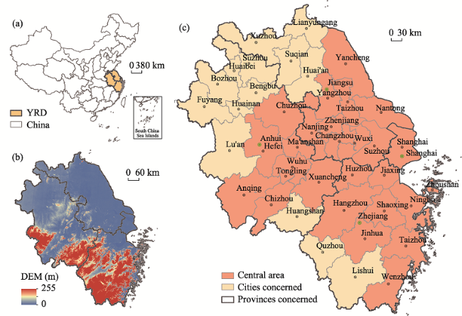
The Yangtze River Delta (YRD) is a region in China with a serious contradiction between economic growth and environmental pollution. Exploring the spatiotemporal effects and influencing factors of air pollution in the region is highly important for formulating policies to promote the high-quality development of urban industries. This study uses the spatial Durbin model (SDM) to analyze the local direct and spatial spillover effects of industrial transformation on air pollution and quantifies the contribution of each factor. From 2008 to 2018, there was a significant spatial agglomeration of industrial sulfur dioxide emissions (ISDE) in the YRD, and every 1% increase in ISDE led to a synchronous increase of 0.603% in the ISDE in adjacent cities. The industrial scale index (ISCI) and industrial structure index (ISTI), as the core factors of industrial transformation, significantly affect the emissions of sulfur dioxide in the YRD, and the elastic coefficients are 0.677 and -0.368, respectively. The order of the direct effect of the explanatory variables on local ISDE is ISCI>ISTI>foreign direct investment (FDI)>enterprise technological innovation (ETI)>environmental regulation (ER)> per capita GDP (PGDP). Similarly, the order of the spatial spillover effect of all variables on ISDE in adjacent cities is ISCI>PGDP>FDI>ETI>ISTI>ER, and the coefficients of the ISCI and ISTI are 1.531 and 0.113, respectively. This study contributes to the existing research that verifies the environmental Kuznets curve in the YRD, denies the pollution heaven hypothesis, indicates the Porter hypothesis, and provides empirical evidence for the formation mechanism of regional environmental pollution from a spatial spillover perspective.

Cite this article

CHEN Yufan , XU Yong , WANG Fuyuan . Air pollution effects of industrial transformation in the Yangtze River Delta from the perspective of spatial spillover[J]. Journal of Geographical Sciences, 2022 , 32(1) : 156 -176 . DOI: 10.1007/s11442-021-1929-6

1 Introduction

Since the reform and opening up, economic development in China has been advancing rapidly. The average annual growth rate of the GDP reached 9.5% from 1978 to 2017, which was hailed as a “growth miracle” (Li, 2017). Rapid economic growth and industrialization processes have been accompanied by excessive resource and energy consumption, especially the use of a large amount of coal in the production process, and this has resulted in serious air pollution in most Chinese cities (Han et al., 2015; Du et al., 2019). Recognizing severe environmental problems, the Chinese government proposed a major policy to promote the harmonious coexistence of humans and nature in the Report of the 19th National Congress of the Communist Party of China (CPC) and incorporated green development into national strategic decisions, which is consistent with the theory of sustainable development promoted globally (Liu and Zhang, 2019; Zhong and Wei, 2019).
Previous studies and theories (e.g., the environmental Kuznets curve, EKC) have indicated that the relationship between the environment and economy is related to scale, structure and technology effects (Copeland and Taylor, 2004). Specifically, the expansion of the industrial scale causes economic agglomeration, and its impact on environmental pollution often has different results. Some scholars have confirmed the positive correlation between environmental pollution and industrial agglomeration through empirical evidence in southern Finland, the European Union, Vietnam and China (Virkanen, 1998; Leeuw et al., 2001; Duc et al., 2007; Xiao and Shen, 2019). This is because industrial agglomeration results in an expanded production scale and increased energy consumption, which creates negative externalities to the environment caused by the crowding effect (Wang, 2018). In addition, the pollution haven hypothesis (PHH) states that developed countries transfer their polluting industries to developing countries, which leads to the low-end industrial structure of developing countries (Liu et al., 2019). However, other scholars have shown that industrial agglomeration can promote the effect of scale economies through the input-output correlation effect and enhance the technology spillover effect (Porter, 1998; Hosoe and Naito, 2006; Li and Wang, 2014). Technological progress and industrial upgrading can improve the utilization rates of energy and resources and reduce the intensity and total amount of pollution emissions (Cole and Elliott, 2003; Zeng and Zhao, 2009; Li, 2018; Chen et al., 2019). Furthermore, high-intensity environmental regulation is very likely to reduce pollution emissions, but it also causes an increase in environmental compliance costs and limits technological innovation (Qi et al., 2015; Funfgelt et al., 2016).
With the development of regional integration, interregional linkages and spatial dependences among cities have been increasing (Cheung and Ping, 2004). An urban agglomeration is an area with close spatial connection and a high level of integration. Consequently, environmental pollution consists not only of local pollution but also of more diffuse spatial spillover pollution, and it exhibits spatial agglomeration characteristics (Becker and Henderson, 2000). Zhou et al. (2017) found that water pollution emissions around the Bohai Sea in China centrally cluster and exhibit an obvious spatial spillover effect. Hou et al. (2018) revealed that the environmental pollution emissions in the Yangtze River Delta (YRD) have a spillover effect at the city level, and there are EKC characteristics between these emissions and per capita income. Regarding the influencing factors, the impact of the industrialization level on environmental pollution in urban agglomerations is the focus of academic circles. Some scholars have confirmed through long-term and multiscale studies that industrial activities play a dominant role in water pollution in urban agglomerations (Wang et al., 2018). An improvement in industrialization aggravates regional water pollutant emissions, and adjacent cities show similar pollution patterns or change characteristics (Zhao et al., 2012; Wilbers et al., 2014). The impact of industrial upgrading on environmental pollution in urban agglomerations is still uncertain. Industrial upgrading can break through geographical and traditional industry limitations by the transfer of production factors and accelerate the optimization of the industrial structure in adjacent areas to thus reduce pollution emissions (Miao and Guo, 2019; Zhang et al., 2019). However, the blind upgrading of industrial structures, as well as the inter-competition between regions, also lead to the irregular flow of production factors in the local and adjacent areas, which results in an imbalance and the spatial spillover of environmental problems (Xiong et al., 2018; Liu et al., 2019; Wang and Meng, 2019).
In general, the environmental spatial effect of industrial development has become a popular research topic, and a large number of spatial econometric models have been applied in studies. However, most studies have focused on a single factor, such as urbanization (Du et al., 2018; Du et al., 2019; Liu et al., 2019), industrialization (Liu et al., 2019; Zhou et al., 2019), and environmental regulation (Qiu et al., 2018; Ran et al., 2019), but what are the spatial spillover effects of industrial transformation (e.g., industrial agglomeration and industrial upgrading) on the environmental pollution in urban agglomerations? This study attempts to expand the research perspective to the entire dynamic process of industrial transformation and development. Its purpose is not only to verify the spatial effect of industrial transformation on regional environmental pollution but also to seek solutions to this regional diffuse pollution from the perspective of industrial transformation. Second, previous studies have mostly focused on cities or regions in northern China where heavy chemical industries are concentrated, and less attention is given to the urban agglomerations in the southeastern coastal areas. The YRD was one of the earliest regions of industrial transformation in China, and it has a strong export orientation and more complete categories of industry. Choosing the YRD as a case area is conducive to regulating the spatial spillover effect of industrial dynamics on regional environmental pollution based on high-quality transformation practices in the YRD. Finally, developing countries have long been regarded as the gathering places of pollution industry transfer due to the relatively low intensity of environmental regulation. This study attempts to combine the PHH with pollution spatial spillover to explore how the scale, structure and technology effects mentioned in the EKC hypothesis work together on environmental pollution in urban agglomerations. Then, this study provides some effective countermeasures for pollution control and sustainable management in the YRD.

2 Theory and methods

2.1 Basic concept

According to new economic growth theory, the regional spillover effect is used to describe the influence of the economic activities in a central region on the economy of other neighboring regions, including the polarization effect and diffusion effect (Huang, 2014). In the field of environmental science, the spatial spillover effect of environmental pollution refers to the impact of local environmental pollution on the ecological environment of adjacent areas, which is essentially a type of mutual conduction relationship of environmental pollution in space (Liu et al., 2015). Spatial spillover is another manifestation of a factor externality, and it is an indirect effect. An externality is an external influence of one economic subject on another. Pigou further developed externalities into the three forms of no externality, negative externality and positive externality on the basis of Marshall’s external economy theory (Demsetz, 2004). When there is a positive externality, because of the existence of a spillover effect, the local income will not be fully owned by the locals, which results in external benefits, such as the improvement of environmental quality; when there is a negative externality, because of damage to the local economy or environment, the adjacent areas must increase the external expenditures to maintain the original development foundation. Industrial development may produce positive or negative externalities to local and adjacent environmental pollution through the effect of scale economies, the structure optimization effect and the technology spillover effect (Ji et al., 2018).

2.2 Research methods

2.2.1 Exploratory spatial data analysis (ESDA)

ESDA can examine data in a more quantitative way than can be achieved by plotting data. Existing studies have shown that the emissions of environmental pollutants have obvious spatial agglomeration characteristics at multiple scales (Chen et al., 2018), and Moran’s I statistic has commonly been used to test the global and local spatial autocorrelations among environmental pollution variables (Liu and Zhang, 2019). The global Moran’s I statistic can be calculated as follows:
${I_{Global}} = \frac{{N\mathop \sum \nolimits_i \mathop \sum \nolimits_j {\omega _{ij}}({x_i} - \bar x)({x_j} - \bar x)}}{{\mathop \sum \nolimits_i \mathop \sum \nolimits_j {\omega _{ij}}\mathop \sum \nolimits_i {{({x_i} - \bar x)}^2}}}$
where N is the total number of spatial units, ωij is the spatial weight matrix, xi and xj are the attribute values of cities i and j, respectively, and $\bar x$ is the average attribute value.
The global Moran’s I has a value in the range of [-1,1]. Global Moran’s I > 0 indicates a positive spatial correlation. Global Moran’s I < 0 indicates a negative spatial correlation. If globl Moran’s I=0, then this indicates spatial randomness.
The local distribution of spatial elements among regions may be atypical and cannot be reflected by global indicators (Anselin, 1995). The local Moran’s I statistic can be used to test the spatial correlation between cities as follows:
$LISA = \frac{{({x_i} - \bar x)}}{{\left[ {\mathop \sum \nolimits_{j = 1}^N {\omega _{ij}}{{({x_j} - \bar x)}^2}/(N - 1)} \right] - \overline {{x^2}} }} \times \mathop \sum \limits_{j = 1}^N {\omega _{ij}}({x_j} - \bar x)$
The local Moran’s I result is often displayed by using XY coordinates, where the X-axis is the standardized value of the actual observation value, and the Y-axis is the spatial lag value, that is, the weighted average value of the area around the observation value (Anselin, 1998). According to the positive and negative characteristics, the following four combinations can be obtained: ① X>0, Y>0, Lisa=X*Y>0, which is a high-high cluster (HH); ② X<0, Y>0, Lisa<0, which is a low value surrounded by high neighboring values (LH); ③ X<0, Y<0, Lisa>0, which is a low-low cluster (LL); and ④ X>0, Y<0, Lisa<0, which is a high value surrounded by low neighboring values (HL).
A spatial weight matrix should be established in a spatial correlation analysis (Feng et al., 2018). An inverse distance-squared spatial weight matrix that uses projected latitudes and longitudes is generated as follows:
${\omega _{ij}} = \left\{ {\begin{array}{*{20}{c}}{0,i = j}\\{\frac{1}{{d_{ij}^2}},i \ne j}\end{array}} \right.$
where dij is the greater Euclidean distance between cities i and j calculated based on the longitude and latitude.

2.2.2 Spatial econometric model

Spatial econometric models can effectively solve the spatial dependence problem that cannot be addressed in a linear regression analysis (Liu et al., 2018). Common spatial regression models include the spatial lag model (SLM), spatial error model (SEM), spatial Durbin model (SDM), etc. (Cheng et al., 2014).
When the error terms of the model are spatially correlated, the model is an SEM, which can be written as follows:
${Y_t} = \alpha {I_N} + \beta {X_t} + \lambda W + \varepsilon,\varepsilon ~N(0,{\delta ^2})$
where Yt is the column vector of the explained variable, Xt is the vector matrix of the explanatory variables, IN is the unit matrix, W is the spatial weight matrix, α is a constant, β is the regression coefficient vector of the explanatory variable, λ is the spatial autocorrelation coefficient between the regression residuals, and ε is the unexplained random error term.
When the spatial dependence of the explained variable is critical to the analysis, which results in spatial correlation, the model can be transformed into an SLM with the following equation:
${Y_t} = \alpha {I_N} + \rho W{Y_t} + \beta {X_t} + \varepsilon,\varepsilon ~N(0,{\delta ^2})$
where ρ is the spatial autoregressive coefficient of the explained variable, and its numerical value reflects the degree of spatial spillover. If ρ is significant, then there is a certain spatial dependence of the explained variable.
The SDM is a more general form of the above two models. The SEM includes the exogenous interaction effects of the error term, while the SLM includes the endogenous interaction effects of the explained variable. Considering both the exogenous and endogenous interaction effects, the estimation results of the SDM are more robust (Elhorst, 2010; Elhorst, 2014), and the basic model can be written as follows:
${Y_t} = \alpha {I_N} + \rho W{Y_t} + \beta {X_t} + \theta W{X_t} + \varepsilon$
where θ is the spatial autoregressive coefficient of the explanatory variable. If the absolute value of θ is large, then the spatial interaction of the explanatory variables is more significant. When θ=0, the SDM can be simplified to an SLM, and when θ+ργ=0, the SDM can be simplified to an SEM.
Using a point estimation to test the spatial spillover effects may result in model estimation bias (Lesage, 2014; Lesage and Sheng, 2014). The total effect of spatial spillover should be decomposed into direct and indirect effects by the partial differential method, and then, the SDM can be converted into the following:
${Y_t} = {({I_N} - \rho W)^{ - 1}}\alpha {I_N} + {({I_N} - \rho W)^{ - 1}}(\beta {X_t} + \theta W{X_t}) + {({I_N} - \rho W)^{ - 1}}{\varepsilon _{it}}$
Then, the partial derivative of each explanatory variable can be calculated as follows:
$\left[ {\frac{{\partial Y}}{{\partial {X_{1K}}}}, \ldots,\frac{{\partial Y}}{{\partial {X_{NK}}}}} \right] = \left[ {\begin{array}{*{20}{c}} {\frac{{\partial {Y_1}}}{{\partial {X_{1K}}}}}& \ldots &{\frac{{\partial {Y_1}}}{{\partial {X_{NK}}}}}\\ \vdots & \ddots & \vdots \\ {\frac{{\partial {Y_N}}}{{\partial {X_{1K}}}}}& \ldots &{\frac{{\partial {Y_N}}}{{\partial {X_{NK}}}}} \end{array}} \right] = {({I_N} - \rho W)^{ - 1}}\left[ {\begin{array}{*{20}{c}} {\begin{array}{*{20}{c}} {\beta 1}&{{W_{12}}{\theta _K}}\\ {{W_{21}}{\theta _K}}&{\beta 2} \end{array}}&{\begin{array}{*{20}{c}} \ldots &{{W_{1N}}{\theta _K}}\\ \ldots &{{W_{2N}}{\theta _K}} \end{array}}\\ {\begin{array}{*{20}{c}} \vdots & \vdots \\ {{W_{N1}}{\theta _K}}&{{W_{N2}}{\theta _K}} \end{array}}&{\begin{array}{*{20}{c}} \ddots & \vdots \\ \ldots &{\beta K} \end{array}} \end{array}} \right]$
where the average of the diagonal coefficient represents the direct effect, which reflects the actual influence of the explanatory variables on the explained variable in the local city, and the average of the nondiagonal coefficient represents the indirect effect, namely, the spatial spillover effect, which represents the average influence of the explanatory variables on the explained variable in the adjacent cities.

2.2.3 Model and variable selection

The causal relationship between the explained and explanatory variables should be considered in the selection of the model control variables.
(1) Explained variable
Pollutants with different attributes have different emission characteristics. The composition of air pollutants is closely related to the energy consumption structure. The main energy source of the YRD is coal, which means that the main air pollutants are sulfur dioxide, nitrogen oxide and particulate matter. Industrial production and domestic fuel combustion are the two main pollution sources of sulfur dioxide. We further compared the emissions of the two sources and found that the amount of sulfur dioxide emitted by industrial production in the YRD was 10.8 times that of daily life and other emissions in 2018. This means that the pollution contribution rate of industrial production was far greater than the pollution contribution rate of daily life. Furthermore, industrial sulfur dioxide emissions (ISDE) are listed as the main emission control indicators by the environmental authorities of the central government and the YRD, which provides a certain time continuity in the statistics. Therefore, we selected ISDE to measure regional industrial pollution.
(2) Core explanatory variables
Industrial transformation is the main feature of economic growth, which includes production scale adjustment, industrial structure upgrading, enterprise layout optimization, etc. The industrial transformation defined in this study includes two aspects. The first refers to quantitative transformation, that is, a city adjusts the industrial scale through agglomeration or transfer to enhance its dominance in the entire region (Miao et al., 2019; Kou et al., 2021). The second aspect refers to quality transformation, that is, the industrial or economic structure of a city moves toward a more profitable development direction, and the production value and creativity are improved (Liu et al., 2019; Meng et al., 2021). Therefore, this study focused on the environmental effects of the industrial scale and structure adjustment and used the industrial scale index (ISCI) and industrial structure index (ISTI), respectively, for quantitative analysis and characterization. The meaning and calculation methods of the ISCI and ISTI are as follows.
① Industrial scale index (ISCI)
An increase in the ISCI represents the growth of the regional economic scale, and location entropy is often used to compare the differences in the ISCI among different cities. When the location entropy is higher, the industrial agglomeration degree is higher (Zhong and Wei, 2019).
$ISC{I_{it}} = \frac{{ID{V_{it}}/GD{P_{it}}}}{{\mathop \sum \nolimits^ ID{V_{it}}/\mathop \sum \nolimits^ GD{P_{it}}}}$
where IDVit is the industrial added value of city i in year t, and GDPit is the total economic production of city i in year t.
② Industrial structure index (ISTI)
The ISTI can be calculated with the comprehensive weighted sum of the industrial advanced index (IAI) and industrial rationalized index (IRI), and the weights of the two indicators are both 50%. Of the indicators, the IAI is expressed as the ratio of the tertiary industry added value to the secondary industry added value, and the IRI is calculated by the Theil index as follows:
$IRI = \mathop \sum \limits_{m = 1}^3 \left[ {\ln \left( {\frac{{{y_{mi}}}}{{{l_{mi}}}}/\frac{{{Y_i}}}{{{L_i}}}} \right) \times \frac{{{y_{mi}}}}{{{Y_i}}}} \right]$
where ymi is the added value of industry m in city i, ${l_{mi}}$ is the employed population of industry m in city i, Yi is the total economic production of city i, and Ll is the total employed population of city i.
(3) Other control variables
In addition to the above core variables, other institutional and economic development factors contribute to environmental pollution. The four control variables selected are as follows. Per capita GDP (PGDP) represents the economic development level of a city. Enterprise technological innovation (ETI) is measured by the number of patent grants, and it affects the quality of industrial development. Foreign direct investment (FDI) is measured by the ratio of the number of foreign-invested companies to the total number of industrial companies and is an important indicator to verify the PHH. Finally, environmental regulation (ER) is measured by the ratio of industrial pollution control investment to industrial added value, and it is used to observe the actual effect of government intervention in the process of pollution management.
Therefore, based on Equation (6), the regression model of this study can be written as follows:
$\begin{array}{c}\ln ISD{E_{it}} = \alpha + \rho \mathop \sum \limits_{j \ne i}^n {\omega _{ij}}\ln ISD{E_{it}} + {\gamma _1}\ln ISC{I_{it}} + {\gamma _2}\ln IST{I_{it}} + {\gamma _3}\ln PGD{P_{it}} + {\gamma _4}\ln ET{I_{it}}\\{\rm{ }} + {\gamma _5}\ln FD{I_{it}} + {\gamma _6}\ln E{R_{it}} + {\theta _1}\mathop \sum \limits_{i \ne j}^N {\omega _{ij}}\ln ISC{I_{it}} + {\theta _2}\mathop \sum \limits_{i \ne j}^N {\omega _{ij}}\ln IST{I_{it}}\\{\rm{ }} + {\theta _3}\mathop \sum \limits_{i \ne j}^N {\omega _{ij}}\ln PGD{P_{it}}{\rm{ + }}{\theta _4}\mathop \sum \limits_{i \ne j}^N {\omega _{ij}}\ln ET{I_{it}} + {\theta _5}\mathop \sum \limits_{i \ne j}^N {\omega _{ij}}\ln FD{I_{it}} + {\theta _6}\mathop \sum \limits_{i \ne j}^N {\omega _{ij}}\ln E{R_{it}} + \varepsilon \end{array}$

3 Study area and data

3.1 Study area

The YRD is one of the most developed urban agglomerations in China. It is located in the lower reaches of the Yangtze River and borders the Yellow Sea and the East China Sea. The terrain is high on the periphery and low in the middle. At the end of 2019, the CPC Central Committee and the State Council issued The Outline of the Yangtze River Delta Regional Integration Development Plan, which designated 41 cities in the YRD, including Shanghai city, provinces of Jiangsu, Zhejiang and Anhui, with a total land area of 358,000 km2. As shown in Figure 1, the following 27 cities represent the central areas, with a total land area of 225,000 km2: Shanghai city; Nanjing, Wuxi, Changzhou, Suzhou, Nantong, Yangzhou, Zhenjiang, Yancheng and Taizhou in Jiangsu Province; Hangzhou, Ningbo, Wenzhou, Huzhou, Jiaxing, Shaoxing, Jinhua, Zhoushan and Taizhou in Zhejiang Province; and Hefei, Wuhu, Maanshan, Tongling, Anqing, Chuzhou, Chizhou and Xuancheng in Anhui Province. All of these central cities have rapidly driven the high-quality development of the YRD. As one of the regions with the most active economic development, the highest degree of openness and the strongest innovation ability in China, the YRD plays an important strategic role in China’s overall modernization and opening pattern. The population agglomeration and urbanization process in the YRD has been rapid. By 2017, the total population had reached 223 million, and the population urbanization rate had reached 69.49%. Moreover, the GDP of the entire YRD is 19.53 trillion yuan, with the proportion of primary industry, secondary industry and tertiary industry being 4.2:41.8:54.0, which accounts for approximately 25% of China’s total economy.
Figure 1 Location of the Yangtze River Delta
With the rapid development of regional integration, environmental losses and ecological damage have become important obstacles for the YRD to achieve the goal of building a world-class urban agglomeration by 2030. In 2017, the total amounts of wastewater discharge, waste gas discharge, industrial solid waste production and domestic waste production in the YRD were 1474.92 million tons, 3.75 million tons, 10.16 million tons and 45.59 million tons, respectively; the land area of the YRD is less than 4% of the entire country, but the proportions of these pollutants are 21.08%, 12.79%, 9.2% and 20.13%, respectively, representing a heavy environmental pollution emission burden per unit area. Due to the spatial proximity and close relationship between cities in the YRD, there is a serious mutual conduction risk of industrial air pollution between cities, which can cause more serious regional air pollution problems. For a long time in the future, water, air and solid waste pollution will be the focus of environmental governance in the YRD.
Against the background of high-quality environmental development, the industrial transformation path of the YRD has gradually shifted from scale reduction and layout optimization to the coexistence of production scale balance, process innovation and technology upgrading, which embodies the changing characteristics of industrial transformation and pollution management in China’s urban agglomerations. Based on the contradiction between industrial development and environmental pollution, the YRD is selected as a case area to analyze the spatiotemporal effect and influencing factors of air pollution from 2008 to 2018 and thus to provide a scientific basis for the realization of regional environmental governance in the integrated development of the YRD.

3.2 Data sources and preprocessing

Environmental pollution and industrial development data were collected from The China Urban Statistical Yearbook (2009-2019), The China Environmental Statistical Yearbook (2009-2019), The City Statistical Yearbook (2009-2019), The Environmental Statistical Bulletin (2009-2019), etc. The industrial patent data of Shanghai, Nanjing, Hangzhou and Ningbo, such as patent applications, patent grants and patents in force, were selected from The Annual Report of Intellectual Property Statistics (2009-2019) provided by the China National Intellectual Property Administration (https://www.cnipa.gov.cn/col/col61/index.html), and the patent authorization data of most other cities were selected from the statistical yearbooks of each city. Then, we combined and sorted the relevant data to obtain the number of valid patents applied for and approved by each city from 2008 to 2018. In addition, to eliminate the impact of price changes and avoid heteroscedasticity and collinearity in the model, we used the GDP deflator index based on 2007 to approximately convert the PGDP and added values of the primary, secondary and tertiary industries of each city over years and then treated all index values logarithmically. Table 1 shows the descriptive statistical results of all experimental data.
Table 1 Descriptive statistics
Variable Obs Mean Std. Dev. Min Max VIF
ln ISDE Industrial Sulfur Dioxide Emissions 451 10.519 0.913 7.563 13.115 -
ln ISCI Industrial Scale Index 451 -0.029 0.220 -1.024 0.479 3.81
ln ISTI Industrial Structure Index 451 -0.769 0.241 -1.895 0.202 2.56
ln PGDP Per Capita GDP 451 10.563 0.719 8.408 11.906 5.39
ln ETI Enterprise Technological Innovation 451 7.905 1.771 2.996 11.496 3.63
ln FDI Foreign Direct Investment 451 -2.996 0.855 -5.369 -1.115 1.85
ln ER Environmental Regulation 451 -1.352 0.448 -2.527 -0.236 1.10
The panel data used in this study, with a time series (T) of 11 and a panel series (N) of 41, are short panel data, and an HT unit root test is required. All variables reject the original assumption of non-stationarity after the first-order difference processing, which indicates that there is no unit root variable (Table 2). Then, the Kao, Pedroni and Westerlund methods were used for cointegration tests. Each statistic is significant at the 1% level, which indicates that there is a long-term stable equilibrium relationship between the variables, and they can be used for a regression analysis. Afterwards, by observing the numerical condition of the AIC, BIC and HQIC, the optimal lag order is determined to be the second order. Through the Ganger test (Table 3), it is found that each explanatory variable is the Granger cause of the explained variable ISDE, that is, there is a causal relationship between them.
Table 2 The results of the HT unit root test
ln ISDE ln ISCI ln ISTI ln PGDP ln ETI ln FDI ln ER
Horizontal sequence 0.660** 0.792 0.711 0.798 0.722 0.774 0.231***
First order difference -0.355*** -0.101*** 0.099*** 0.048*** -0.045*** -0.007*** -0.247***

Notes: ***, **, and * represent significance at 1%, 5%, and 10%, respectively.

Table 3 The results of the Granger test
Granger causality test of hypothesis a F-Statistic Granger causality test of hypothesis b F-Statistic
ISDE-ISCI 10.796*** ISCI-ISDE 5.946***
ISDE-ISTI 12.818*** ISTI-ISDE 15.742***
ISDE-PGDP 2.152** PGDP-ISDE 2.839***
ISDE-ETI 7.911*** ETI-ISDE 4.615***
ISDE-FDI 9.038*** FDI-ISDE 9.721***
ISDE-ER 4.594*** ER-ISDE 5.359***

Notes: a—the explanatory variable does not Granger-cause the explained variable. b—the explained variable does not Granger-cause the explanatory variable. ***, **, and * represent significance at 1%, 5%, and 10%, respectively.

To assess the spatial clustering and distribution of the different variables more clearly, all variables were visualized on a map (Figure 2). The distribution of indicators in the YRD shows an obvious spatial imbalance, and it forms two heterogeneous regions in the northeast and southwest. Of these areas, the environmental pollution in the cities in the northeast is relatively heavy, and the level of economic and social development, such as industrial development and technological innovation, is higher, while the southwestern cities show the opposite.
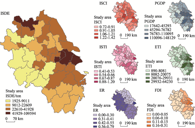
Figure 2 Spatial distributions of the variables - ISDE, ISCI, ISTI, PGDP, ETI, FDI and ER

4 Results

4.1 Spatial correlation test of ISDE

Global Moran’s I of the ISDE in the YRD from 2008 to 2018 is calculated according to equation (1), as listed in Table 4. Based on the geographical inverse distance-squared matrix, the ISDE from 2008 to 2018 rejects the original hypothesis of no spatial autocorrelation at the different significance levels, and the correlation coefficient is significantly positive each year, which indicates that there is a significant positive spatial correlation of industrial air pollution in the YRD. Thus, cities with more serious air pollution tend to be adjacent in space, and cities with lower emissions are also adjacent in space. From the interannual variation in the global Moran’s I, although it has a certain volatility, the overall value shows a weakening trend, which suggests that the spatial autocorrelation of ISDE among different cities in the YRD is decreasing, and the spatial difference of regional air pollution is expanding.
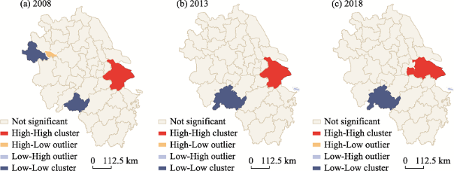
Table 4 Global Moran’s I of the ISDE in the Yangtze River Delta from 2008 to 2018
Year 2008 2009 2010 2011 2012 2013
Moran’s I 0.201** 0.191** 0.223*** 0.257*** 0.258*** 0.254***
Year 2014 2015 2016 2017 2018
Moran’s I 0.206*** 0.207*** 0.231*** 0.236** 0.227***

Notes: ***, **, and * represent significance at 1%, 5%, and 10%, respectively.

Local autocorrelation tests of ISDE in 2008, 2013 and 2018 are carried out according to Equation (2). The results show that the local spatial distribution of industrial air pollution is mainly represented by HH and LL agglomerations. From the perspective of specific city distribution patterns (Figure 3), HH clusters are mainly concentrated in Shanghai, southern Jiangsu and northern Zhejiang, which have a high level of economic development and a large industrial scale. The industrial clusters are dominated by industries with high energy consumption and high pollution, such as equipment manufacturing, pharmaceutical chemistry, papermaking and textiles. LL clusters are located in the southwestern cities of Anhui Province, which focuses on the development of the cultural and tourism industry, and the industrial economy is not prominent. For example, Huangshan city, as an important birthplace of Hui culture, has actively developed its tertiary industry through tourism as the main industry. The contribution rate of manufacturing industry to the city’s economy is only 29.2%, and the pollution emissions caused by industrial production are relatively low.
Figure 3 Cluster maps of the ISDE in the Yangtze River Delta

4.2 Spatial regression results based on the SDM

The maximum likelihood is used for the regression analysis in the software platform stata15. According to the results of the Hausman test, the fitting effect of the fixed-effect model is better than that of the random-effect model. The results of the Wald and likelihood ratio tests both significantly reject the original assumption that the SDM can be simplified as an SLM or SEM, i.e., the SDM attains the best fitting effects. The estimation results of these three models are summarized in Table 5. Based on the geographic inverse distance-squared matrix, the regression results of the SDM show that the spatial autoregressive coefficient $\rho$ is significantly positive at the 1% level, and every 1% increase in ISDE locally will lead to a 0.603% average increase in the ISDE in adjacent cities. Combined with the spatial autocorrelation analysis in the previous section, this indicates that there are spatial agglomeration and positive spillover effects of industrial air pollution emissions in the YRD. Cities with close geographical distances interact with one another, and industrial air pollutants form and diffuse among different cities in urban agglomerations.
Table 5 Results of different spatial regression estimations in the Yangtze River Delta
Variables SEM SLM SDM
ln ISCI 0.574*** 0.560*** 0.677***
ln ISTI -0.505*** -0.262* -0.368**
ln PGDP 0.027 0.230* 0.045
ln ETI -0.136*** -0.090** -0.148***
ln FDI -0.154** -0.233*** -0.170**
ln ER -0.088* -0.059 -0.027
W*ln ISCI 0.296
W*ln ISTI 0.261
W*ln PGDP -0.573*
W*ln ETI 0.284***
W*ln FDI 0.458***
W*ln ER 0.009
$\rho$ 1.102* 0.603***
R2 0.249 0.028 0.418
sigma2_e 0.062*** 0.058*** 0.061***
Wald test 28.73***
L-ratio test 172.89***
Hausman test 51.45***

Notes: ***, **, and * represent significance at 1%, 5%, and 10%, respectively.

Furthermore, an increase in the ISCI by 1% in the YRD will lead to a 0.677% average increase in ISDE. Because the local and adjacent cities in the YRD are usually in the same economic division system, with similar industrial structures, production technologies and capital markets, the action mechanism on the ecological environment is also similar. For example, the manufacturing industry is highly concentrated in the central area of the YRD, and it can trigger industrial production activities with high energy consumption through the agglomeration effect, which directly increases regional air pollutant emissions.
In contrast, every 1% increase in the ISTI will reduce ISDE by 0.368%. Industrial structure adjustment drives the improvement of local production efficiency and the technological innovation level. In the YRD, industrial structure adjustment not only means a simple transfer from the secondary industry to the tertiary industry but also extends the low-end equipment manufacturing industry to the high-end industrial chain, such as biomedicine and advanced equipment manufacturing, which greatly reduces production energy consumption and industrial pollution.
For every 1% increase in PGDP, ISDE will increase by 0.045%. This shows that the YRD is still in the stage of a gradual reduction of environmental quality with economic growth, and the economic growth mode at the cost of environmental pollution has not completely changed. Technical and policy variables such as EIT, FDI and ER have negative effects on the ISDE in the YRD, and the correlation coefficients are -0.148, -0.170 and -0.027, respectively. Through the improvement of production technology, the development of the environmental access threshold and the enhancement of the ER intensity, innovative elements such as talent, capital and information have a positive impact on the cleaner production of urban enterprises through the industrial chain.

4.3 Decomposition of the spatial effects

According to the WX coefficient in Table 5, the explanatory variables all show significant exogenous interaction effects. To explain the spatial autoregressive coefficient of the SDM more specifically, the spatial effects of industrial transformation on air pollution can be decomposed according to equation (8), and the results are summarized in Table 6.
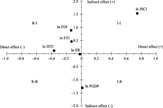
Table 6 Direct, indirect and total effects of the SDM in the Yangtze River Delta
Variables Direct effect Indirect effect Total effect
ln ISCI 0.745*** 1.531* 2.530*
ln ISTI -0.367** 0.113 -0.254
ln PGDP 0.010 -1.306* -1.296**
ln ETI -0.134*** 0.461** 0.328*
ln FDI -0.139** 0.886*** 0.746**
ln ER -0.022 -0.019 -0.041

Notes: ***, **, and * represent significance at 1%, 5%, and 10%, respectively.

The direct effect represents the influence of the explanatory variables on the explained variables in the local city. The contribution order of different explanatory variables is ISCI> ISTI#>FDI#>ETI#>ER#>PGDP, where $#$ represents a negative effect, and the ISCI, ISTI, ETI and FDI are significant at the different confidence levels. The indirect effect, namely, the spatial spillover effect, represents the average influence of the explanatory variables on the explained variables in adjacent cities. The contribution ranking is ISCI>PGDP#>FDI> ETI>ISTI>ER#, and only the ISTI and ER fail to pass the significance test. Among them, the ISCI, ISTI, ETI and FDI exhibit positive environmental spillover effects, while PGDP and ER have negative environmental spillover effects. To further reflect the spatial interaction of different explanatory variables on the air pollution of local and adjacent cities, the direct effect and spatial spillover effect are taken as the X-axis and Y-axis, respectively, and four quadrants are divided using Origin9.3 software (Figure 4). The four impact patterns are de-fined as follows: ① I-I: a simultaneous increase in the ISDE in local and adjacent cities; ② R-I: a reduction in the ISDE in the local city but an increase in the ISDE in adjacent cities; ③ I-R: an increase in the ISDE in the local city but a reduction in the ISDE in adjacent cities; and ④ R-R: a simultaneous reduction in the ISDE in local and adjacent cities.
Figure 4 Four impact patterns of the explanatory variables
The ISCI is located in the I-I quadrant. Combined with the decomposition coefficient value in Table 6, the direct and indirect effects of the ISCI are 0.745 and 1.531, respectively, which are significant at the 1% and 10% levels. This result means that each 1% increase in the local ISCI will lead to a 0.745% and 1.531% increase in the ISDE in local and adjacent cities, and the spatial spillover effect of the ISCI is obvious. The industrial structure of the YRD is still dominated by secondary industry, and the proportion of polluting industries, such as chemical materials, nonmetallic minerals and metal smelting, remains high. The expansion of the production scale of these high-polluting industries will inevitably lead to the aggravation of local air pollution. Moreover, the distribution of production factors in the YRD often has the characteristics of spatial agglomeration. In Suzhou, Wuxi and Changzhou, a large number of industrial parks have biomedicine and equipment manufacturing as the main industries, and the industrial chain runs through these three cities. The cluster development mode between cities makes the scale effect of industrial agglomeration more prominent, which leads to the spatial spillover effect of promoting emissions of air pollutants from adjacent cities.
The ISTI is located in the R-I quadrant, which indicates that every 1% increase in the ISTI reduces the local ISDE by 0.367% but increases the ISDE of adjacent cities by 0.113%. In the YRD, especially in core cities such as Shanghai, Suzhou and Hangzhou, the purpose of industrial structure adjustment is more to realize the balance between the manufacturing and service industries and complete industrial upgrading within the manufacturing industry. Under such targeted control, local cities introduce more industries at the high end of the industrial chain and control pollutant emissions from the source through technical effects. Moreover, some high-energy consumption and high-pollution industries in core cities will be transferred to adjacent cities, and the scale of these eliminated industries will be forced to grow continuously, which will directly aggravate pollutant emissions.
In terms of the spatial spillover effect of the other control variables, PGDP is in the I-R quadrant, and for every 1% increase in GPDP, the ISDE in adjacent cities will decrease by 1.306%, which implies that urban economic agglomeration has a positive externality and drives improvements in the green production efficiency of surrounding cities. Both ETI and FDI are located in the R-I quadrant, and the direct effect is significantly negative, while the spatial spillover effect is significantly positive. Thus, ETI and FDI have a reduction effect on the ISDE of the local city but aggravate the ISDE of adjacent cities to varying degrees. The distribution of innovation factors in the YRD is not balanced. After the main body of innovation flows into the central city, it will inevitably lead to the reduction of innovation factors in adjacent cities, which will result in differing air pollution between the surrounding cities. The spatial spillover effect of FDI is related to the quantity and quality of foreign investment. At present, the negative externality of scale spillover is still stronger than the positive externality of technology spillover in the YRD. Therefore, local cities have changed their mode of production and industrial structure by attracting foreign capital, but traditional industries are transferred, which aggravates the air pollutant emissions of adjacent cities. ER is located in the R-R quadrant, and the coefficients of the direct and indirect effects are -0.022 and -0.019, respectively. Under the policy constraints of high-quality environmental development, the high standard ER in the YRD will stimulate enterprises to promote technological innovation to offset the cost of environmental emission reduction to achieve a win-win situation between environmental protection and economic development. Moreover, ER has a certain radiation range (Liu et al., 2021). There is ER competition in adjacent cities. Adjacent cities will follow suit and strengthen their regulation intensity, resulting in the simultaneous reduction of industrial emissions.

5 Conclusion, implications and future directions

5.1 Conclusion and discussion

In this study, 41 prefecture-level cities in the YRD in China were adopted as spatial units, and ESDA and SDM were used to test the spatial spillover effects of industrial transformation on industrial air pollution in urban agglomerations. The findings are as follows.
First, there is a significant spatial autocorrelation of air pollution in the YRD, and the agglomeration characteristics of the cities in the eastern YRD are obvious. According to the spatial regression coefficient, a 1% increase in ISDE locally will lead to a synchronous increase of 0.603% in the ISDE of adjacent cities, which suggests that ISDE has a significant positive spatial effect at the scale of urban agglomeration. This conclusion is similar to the research results of Liu et al. (2018) in the Bohai Rim region, where it was shown that PM2.5 emissions have significant spatial agglomeration and diffusion, and there is a positive interaction between cities. Our study confirms that regardless of the industrial development stage or mode of urban agglomeration, pollutant diffusion from local to adjacent areas is objective. As air mobility is large, pollutant emissions easily spread between regions, which leads to cross-regional air pollution problems. Moreover, the distribution of economic and social production factors is spatially related. For example, companies, capital investment, etc. tend to have spatial convergence. The agglomeration of high energy-consuming and high-polluting companies is likely to cause high-emission air pollution problems, while the agglomeration of green production factors will reduce regional air pollutant emissions, both of which cause air pollutant emissions to have a significant spatial spillover effect.
Second, for every 1% increase in the ISCI and ISTI, the ISDE of the entire YRD will increase by 0.677% and decrease by 0.368%, respectively, with a significant spatial effect. Previous studies have shown that economic agglomeration has a different degree of spatial correlation with pollutant emissions, and it leads to environmental degradation at the watershed and provincial scales (Liu et al., 2017; Liu et al., 2014). High-quality industrial transformation is conducive to improving labor productivity, promoting stricter environmental regulation and reducing pollution (Hosoe et al., 2006; Wang et al., 2018). Our study shows that in urban agglomerations with convenient transportation and capital circulation, such as the YRD, the process of industrial economic agglomeration will also aggravate air pollution. The scale of the traditional manufacturing industry has not been significantly reduced in the current transformation stage; therefore, the problem of high pollution emissions has not been completely solved. However, under the guidance of high-quality environmental development policies, the industrial structure of the YRD is gradually changing to green and digital, and the low-energy production mode has restrained pollutant emissions to a certain extent.
Third, the air pollution effect of industrial transformation can be decomposed into the local direct effect and the spatial spillover effect. The contribution order of the direct effect is ISCI>ISTI>FDI>ETI>ER>PGDP, and the contribution order of the spatial spillover effect is ISCI>PGDP>FDI>ETI>ISTI>ER. All explanatory variables can be divided into four impact patterns, namely, I-I, R-I, I-R and R-R, where I means increasing emissions, and R means reducing emissions. The current study further decomposes industrial transformation into industrial agglomeration and structure adjustment. Through an SDM analysis, it is found that industrial transformation does not blindly promote pollutant emissions, and not all factors produce significant spatial spillover effects. We should focus on the core factors with strong significance, such as industrial agglomeration, to alleviate the process of environmental stress. The EKC hypothesis proposes that economic growth affects environmental quality in three ways, specifically, through scale, technology and structure effects (Copeland and Taylor, 2004). The traditional EKC takes the level of economic development as the independent variable to fit the curve (Zhou et al., 2019), but an increasing number of studies take the level of industrial development as the main variable in theoretical discussions (He et al., 2016). In this study, to explain the rationality of the EKC hypothesis from different aspects, the ISCI and PGDP are selected to measure the scale effect, and the ISTI is selected to measure the structure effect. In addition, ETI and FDI are selected to measure the technology effect. Through an empirical analysis of the YRD, it is verified that the scale effect worsens the environment, while the structure and technology effects improve the environment.
Finally, the spatial spillover effect of industrial transformation on air pollution in the YRD is also affected by foreign investment, innovation, ER and other factors, and these effects should not be completely ignored. Some scholars have studied the PHH in ASEAN, Europe and Latin America and have verified the validity of the PHH by analyzing the distribution law and externality of FDI (Mulatu et al., 2010; Baek, 2016; Sapkota et al., 2017). To explore whether the PHH is true in the YRD, this study adds the FDI index to the control variable. The results show that the spatial coefficient of FDI is -0.170, which is negative and significant at the 1% level; thus, FDI results in emission reductions, and the PHH does not hold in the YRD. The reason is that the YRD has a high intensity of ER, which consists of a strict environmental protection access system for foreign-invested enterprises and open information evaluation standards concerning the environmental behavior of all enterprises. Most of the foreign-invested enterprises choose to invest in industries at the back-end of the industrial chain with low pollution. This type of investment brings more technological progress and innovation upgrading, which to a certain extent inhibits the negative impact of FDI on the regional environment. In addition, by introducing the ER index, it can be found that Porter’s hypothesis is more suitable for the YRD, which is an area with high requirements of ER and a relatively successful industrial transformation. The innovation effect of ER has brought a win-win situation between economic growth and environmental protection.

5.2 Implications

Under the guidance of a high-quality environmental development strategy, the YRD should adhere to the green and sustainable economic growth mode, strengthen the positive roles of the technology and structure effects, and weaken the negative scale effect. The YRD should give attention to the importance of industrial agglomeration, industrial transfer and industrial transformation in the process of economic development and the spatial interaction between them and air pollution emissions to address the environmental problems caused by the traditional industrial transformation mode.
First, the YRD needs to optimize the industrial transformation path with a focus on structural emission reduction. The YRD should give attention to the flow direction of foreign investment and increase the investment proportion of high-end technology industries and other environmentally friendly industries by setting higher market access thresholds and other ER means. In addition, the YRD needs to eliminate traditional enterprises with high pollution and backward technology, speed up the development of modern service and strategic emerging industries, and actively play the positive externality of the scale and structure effects through industrial renewal.
Second, the YRD should achieve ultralow emission transformation with a focus on technology upgrading. The measures include improving the treatment of industrial waste gas from pollution-intensive industries, such as chemical materials, metal smelting byproducts and nonmetallic mineral products, and gradually implementing specific emission limits for air pollutants in the national emission standards for these industries. At the same time, the YRD should carry out advanced technologies and cleaner production concepts in key industries, such as steel and cement, increase environmental protection investment, and improve the positive externality of the technology effect.
Third, a regional joint prevention and control mechanism focused on spillover governance should be formed. With the YRD as the carrier, the negative spatial spillover effect in pollution control should be eliminated. Local and adjacent cities should reach a consensus on pollution emission standards and total emission reductions, actively promote policy coordination and resource sharing among cities, and establish deep-level emission reduction modes for the entire YRD, such as environmental access, pollution payments, and cross-border early warnings.

5.3 Limitations and future directions

By introducing the factors of industrial agglomeration and structure adjustment, our study systematically discusses the relationship and impact mechanism between industrial transformation and environmental pollution in urban agglomerations from the perspective of spatial spillover. It is concluded that the EKC hypothesis can still reasonably explain the spatial interaction between industrial transformation and air pollution emissions under different transformation paths through scale, structure and technology effects. This empirical study of typical regions in the YRD also provides case evidence for controlling the spatial effect of environmental pollution by using the industrial development in developing countries. However, economic development and environmental quality vary greatly among different regions of China. The YRD is representative of the developed regions in China. The conclusions are related to the characteristics of this region. In the future, the SDM can be applied to other regions to verify the applicability of the model and better reveal the regional differences in the environmental spatial effects. In addition, environmental pollution mainly focuses on air pollution, which has strong mobility. Other common environmental pollutants, such as wastewater and solid waste, have not been studied in depth here and can be further discussed in the future. Furthermore, this study only divides the industry into primary, secondary and tertiary industries and does not subdivide the next level of industry sectors. The environmental spatial effects brought by the transformation of these various subindustries are also different, which is worthy of in-depth research.
[1]
Anselin L, 1988. Spatial Econometrics:Methods and Models. Springer Sci. Business Media.

[2]
Anselin L, Florax RJ, 1995. Small Sample Properties of Tests for Spatial Dependence in Regression Models: Some Further Results, New Directions in Spatial Econometrics. Springer. Springer, 21-74.

[3]
Baek J, 2016. A new look at the FDI-income-energy-environment nexus: Dynamic panel data analysis of ASEAN. Energy Policy, 91: 22-27.

DOI

[4]
Becker R, Henderson V, 2000. Effects of air quality regulations on polluting industries. Journal of Political Economy, 108(2): 379-421.

DOI

[5]
Chen J, Xu C, Li K et al., 2018. A gravity model and exploratory spatial data analysis of prefecture-scale pollutant and CO2 emissions in China. Ecological Indicators, 90: 554-563.

DOI

[6]
Chen Y, Lu J, Yu P, 2019. Does technology innovation reduce environmental pollution? Empirical research based on 285 Chinese cities. Journal of Xi’an Jiaotong University (Social Sciences), 39(1): 73-84. (in Chinese)

[7]
Cheng Y, Wang Z, Ye X et al., 2014. Spatiotemporal dynamics of carbon intensity from energy consumption in China. Journal of Geographical Sciences, 24(4): 631-650.

DOI

[8]
Cheung K Y, Ping L, 2004. Spillover effects of FDI on innovation in China: Evidence from the provincial data. China Economic Review, 15(1): 25-44. (in Chinese)

DOI

[9]
Cole M A, Elliott R J R, 2003. Determining the trade-environment composition effect: The role of capital, labor and environmental regulations. Journal of Environmental Economics & Management, 46(3): 363-383.

[10]
Copeland B R, Taylor M S, 2004. Trade, growth, and the environment. Journal of Economic Literature, 42(1): 7-71.

DOI

[11]
Demsetz H, 2004. The core disagreement between Pigou, the profession, and Coase in the analyses of the externality question. European Journal of Political Economy, 12(4): 565-579.

DOI

[12]
Du Y, Sun T, Peng J et al., 2018. Direct and spillover effects of urbanization on PM2.5 concentrations in China's top three urban agglomerations. Journal of Cleaner Production, 190: 72-83.

DOI

[13]
Du Y, Wan Q, Liu H et al., 2019. How does urbanization influence PM2.5 concentrations? Perspective of spillover effect of multi-dimensional urbanization impact. Journal of Cleaner Production, 220: 974-983.

DOI

[14]
Duc T A, Vachaud G, Bonnet M P et al., 2007. Experimental investigation and modelling approach of the impact of urban wastewater on a tropical river: A case study of the Nhue River, Hanoi, Viet Nam. Journal of Hydrology, 334(3): 347-358.

DOI

[15]
Elhorst J P, 2010. Applied spatial econometrics: Raising the bar. Spatial Economic Analysis, 5(1): 9-28.

DOI

[16]
Elhorst J P, 2014. Spatial Regressions: From Cross-Sectional Data to Spatial Panels. Heidelberg: Springer, New York Dordrecht London.

[17]
Grossman G M, Krueger A B, 1995. Economic growth and the environment. NBER Working Papers, 110(2): 353-377.

[18]
Han L, Zhou W, Li W, 2015. City as a major source area of fine particulate (PM2.5) in China. Environmental Pollution, 206: 183-187.

DOI

[19]
Hao Y, Zheng S Q, Zhao M Y et al., 2020. Reexamining the relationships among urbanization, industrial structure, and environmental pollution in China: New evidence using the dynamic threshold panel model. Energy Reports, 6: 28-39.

[20]
Hosoe M, Naito T, 2006. Trans-boundary pollution transmission and regional agglomeration effects. Papers in Regional Science, 85(1): 99-120.

DOI

[21]
Hou B, Ma R F, Dou S M, 2018. Environmental scale effects on economic development of urban agglomeration in Yangtze River Delta. Journal of Ningbo University (Natural Science & Engineering Edition), 31(2): 108-114. (in Chinese)

[22]
Huang X Y, 2014. The analysis of spatial spillover effects in regional tourism economic: A case study on Sichuan province[D]. Chengdu: Southwestern University of Finance and Economics. (in Chinese)

[23]
Ji Y J, Shao H Z, 2018. The impact of industrial agglomeration on environmental pollution: Aggravation or restraint. Economy and Management, 32(3): 59-64. (in Chinese)

[24]
Jia Z, Qiang W, Wang Y et al., 2020. The spatial characteristics and spatial effect of industrial pollution agglomeration in Lanzhou-Xining Urban Agglomeration. Economic Geography, 40: 68-75, 84.

[25]
Kou D, 2021. A study on the relationship between industrial agglomeration mode and environmental pollution. Economic Survey, 38(4): 73-82. (in Chinese)

[26]
Leeuw F A A M D, Moussiopoulos N, Sahm P et al., 2001. Urban air quality in larger conurbations in the European Union. Environmental Modelling & Software, 16(4): 399-414.

[27]
Lesage J P, 2014. Spatial econometric panel data model specification: A Bayesian approach. Social Science Electronic Publishing, 9: 122-145.

[28]
Lesage J P, Sheng Y, 2014. A spatial econometric panel data examination of endogenous versus exogenous interaction in Chinese province-level patenting. Journal of Geographical Systems, 16(3): 233-262.

DOI

[29]
Li J, 2017. Urbanization, institutional arrangement and regional environmental pollution[D]. Changsha: Hunan University. (in Chinese)

[30]
Li L Z, Fu Z Q, Wang Y H et al., 2017. Empirical study on manufacturing transfer and environmental impacts in Jing-Jin-Ji region. Research of Environmental Sciences, 30(12): 1813-1821.

[31]
Li Q, 2018. Has industrial upgrading promoted the ecological environment optimization of the Yangtze River Economic Belt? Based on the urban panel data of 108 cities. Finance and Trade Research, 29(12): 39-47.

[32]
Li S, Wang S, 2014. An empirical test of the impact of industrial agglomeration on China’s industrial pollution emissions. Statistics & Decision, (8): 128-130. (in Chinese)

[33]
Liu F, Liu C, 2019. Regional disparity, spatial spillover effects of urbanization and carbon emissions in China. Journal of Cleaner Production, 241: 1-10.

[34]
Liu G Y, Yang Z F, Tang Y C et al., 2017. Spatial correlation model of economy-energy-pollution interactions: The role of river water as a link between production sites and urban areas. Renewable & Sustainable Energy Reviews, 69: 1018-1028.

[35]
Liu H, Fang C, Huang J et al., 2018. The spatial-temporal characteristics and influencing factors of air pollution in Beijing-Tianjin-Hebei urban agglomeration. Acta Geographica Sinica, 73(1): 177-191. (in Chinese)

[36]
Liu H, Liu B, Zheng S, 2019. The impact of environmental regulation on manufacturing upgrading. China Soft Science, (5): 40-52. (in Chinese)

[37]
Liu H J, Liu C M, Yang Q, 2015. Spatial spillover and the source of environment pollution: Empirical study on the perspective of network analysis. Economist, (10): 28-35.

[38]
Liu M, Chen H, Xu Y, 2021. Study on the effect of environmental regulation on industrial pollution spillover: Empirical evidence from 285 cities nationwide. Economic Geography, 41(2): 194-202. (in Chinese)

[39]
Liu M F, Xie H J, 2014. The convergence research of economy aggregation and pollution aggregation among China's provinces. Economic Geography, 34(4): 25-32. (in Chinese)

[40]
Liu N, Sun Y, Tang J et al., 2019. The environmental effects of pollution-intensive industry agglomeration based on the perspective of spatial spillover. Acta Scientiae Circumstantiae, 39(7): 2442-2454. (in Chinese)

[41]
Liu S, Zhang J, 2019. Space distance, spillover effect and environmental pollution. Inquiry into Economic Issues, (1): 149-158. (in Chinese)

[42]
Liu X, Li L, Ge J et al., 2019. Spatial spillover effects of environmental regulations on China’s haze pollution based on static and dynamic spatial panel data models. Polish Journal of Environmental Studies, 28(4): 2231-2241.

DOI

[43]
Meng H, Zhang M, 2021. Environmental pollution, intensity of technological innovation and transformation and upgrading of industrial structure. Modern Economic Science, 43(4): 65-76. (in Chinese)

[44]
Miao J, Guo H, 2019. The influence mechanism of industrial cooperative agglomeration on environmental pollution: An empirical study based on panel data of urban agglomeration in Yangtze River Delta. Modernization of Management, 39(3): 76-82. (in Chinese)

[45]
Mulatu A, Gerlagh R, Rigby D et al., 2010. Environmental regulation and industry location in Europe. Environmental & Resource Economics, 45(4): 459-479.

[46]
Pan W, 2012. Regional linkages and spatial spillovers of economic growth in China. Economic Research Journal, (1): 54-65.

[47]
Porter M E, 1998. Clusters and the new economics of competition. Harvard Business Review, 76(6): 77.

PMID

[48]
Qiu J L, Pan A L, Zhang G Z, 2018. Formal environmental regulation, informal environmental regulation and green merger and acquisition of heavily polluted enterprises. Social Sciences in Guangdong, (2): 51-59. (in Chinese)

[49]
Ran Q, Xu L, 2019. Environmental regulation, inter-provincial industrial transfer and pollution spillover effect: Based on spatial Durbin model and dynamic threshold panel model. East China Economic Management, 33(7): 5-13. (in Chinese)

[50]
Sapkota P, Bastola U, 2017. Foreign direct investment, income, and environmental pollution in developing countries: Panel data analysis of Latin America. Energy Economics, 64: 206-212.

DOI

[51]
Shao S, Yang Z, Yang L et al., 2019. Can China’s energy intensity constraint policy promote total factor energy efficiency? Evidence from the industrial sector. The Energy Journal, 40(4): 101-128.

[52]
Tobler W R, 1979. Lattice tuning. Geographical Analysis, 11(1): 36-44.

DOI

[53]
Virkanen J, 1998. Effect of urbanization on metal deposition in the bay of Töölönlahti, Southern Finland. Marine Pollution Bulletin, 36(9): 729-738.

DOI

[54]
Wang B, Hong G, Qin T et al., 2019. Factors governing the willingness to pay for air pollution treatment: A case study in the Beijing-Tianjin-Hebei region. Journal of Cleaner Production, 235: 1304-1314.

DOI

[55]
Wang J, 2018. Empirical research on the impact of industrial agglomeration on environmental pollution: Based on the panel data of prefecture-level city[D]. Hangzhou: Zhejiang University. (in Chinese)

[56]
Wang S, Meng D, 2019. Study on the environmental effects of industrial transformation under the haze spillover: Empirical analysis based on Beijing-Tianjin-Hebei and 31 surrounding cities. Ecological Economy, 35(1): 144-149.

[57]
Wang X, Li Y, 2020. Research on measurement and improvement path of industrial green development in China: A perspective of environmental welfare efficiency. Environmental Science and Pollution Research, 27: 42738-42749.

DOI

[58]
Wang X, Tian G, Yang D et al., 2018. Responses of PM2. 5 pollution to urbanization in China. Energy Policy, 123: 602-610. (in Chinese)

DOI

[59]
Wang Z, Jia H F, Xu T et al., 2018. Manufacturing industrial structure and pollutant emission: An empirical study of China. Journal of Cleaner Production, 197(1): 462-471.

DOI

[60]
Wu H, Li Y, Hao Y et al., 2020. Environmental decentralization, local government competition, and regional green development: evidence from China. Science of The Total Environment, 708: 135085.

DOI

[61]
Xiao Z, Shen Z, 2019. The temporal and spatial evolution of population & industrial agglomeration and environmental pollution and the relevance analysis. Journal of Arid Land Resources and Environment, 33(2): 3-10. (in Chinese)

[62]
Xiong L, de Jong M, Wang F et al., 2018. Spatial spillover effects of environmental pollution in China’s Central Plains Urban Agglomeration. Sustainability, 10(4): 994.

DOI

[63]
Zeng D Z, Zhao L, 2009. Pollution havens and industrial agglomeration. Journal of Environmental Economics & Management, 58(2): 141-153. (in Chinese)

[64]
Zhao X, Huang X, Liu Y, 2012. Spatial autocorrelation analysis of Chinese inter-provincial industrial chemical oxygen demand discharge. International Journal of Environmental Research and Public Health, 9: 2031-2044.

DOI

[65]
Zhong J, Wei Y, 2019. Spatial effects of industrial agglomeration and open economy on pollution abatement. China Population, Resources and Environment, 29(5): 98-107. (in Chinese)

[66]
Zhou K, Fan J, Liu H C, 2017. Spatiotemporal patterns and driving forces of water pollutant discharge in the Bohai Rim Region. Progress in Geography, 36(2): 171-181. (in Chinese)

[67]
Zhou K, Liu H C, Wang Q, 2019. The impact of economic agglomeration on water pollutant emissions from the perspective of spatial spillover effects. Journal of Geographical Sciences, 29(12): 2015-2030.

DOI

Outlines

/