Method for UAV-based 3D topography reconstruction of tidal creeks

  • ZHANG Xuhui , 1, 2 ,
  • LI Huan , 1, 2, * ,
  • GONG Zheng 1, 2 ,
  • ZHOU Zeng 1, 2 ,
  • DAI Weiqi 3 ,
  • WANG Lizhu 4 ,
  • Samuel DARAMOLA 2
Expand
  • 1. Jiangsu Key Laboratory of Coast Ocean Resources Development and Environment Security, Hohai University, Nanjing 210098, China
  • 2. College of Harbor, Coastal and Offshore Engineering, Hohai University, Nanjing 210098, China
  • 3. Yellow River Institute of Hydraulic Research, YRCC, Zhengzhou 450003, China
  • 4. College of Marine Science and Engineering, Nanjing Normal University, Nanjing 210046, China
* Li Huan, PhD and Associate Professor, E-mail:

Zhang Xuhui (1996-), Master Candidate, specialized in tidal flats and remote sensing, E-mail:

Received date: 2021-03-05

  Accepted date: 2021-08-17

  Online published: 2022-02-25

Supported by

China National Funds for Distinguished Young Scientists(51925905)

National Natural Science Foundation of China(41401371)

Copyright

Copyright reserved © 2021. Office of Journal of Geographical Sciences All articles published represent the opinions of the authors, and do not reflect the official policy of the Chinese Medical Association or the Editorial Board, unless this is clearly specified.

Abstract

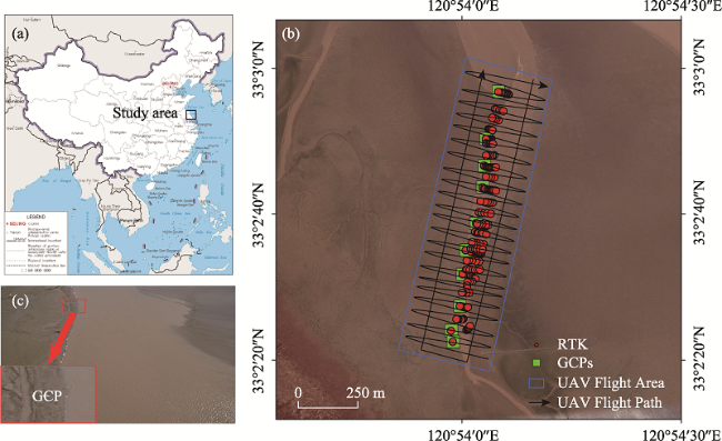
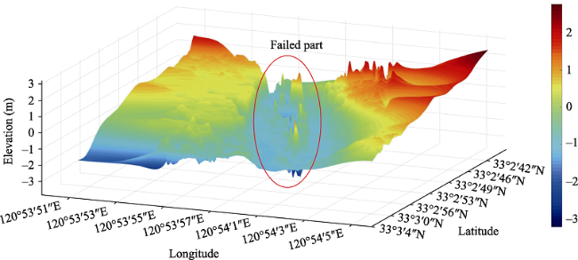
It is common to obtain the topography of tidal flats by the Unmanned Aerial Vehicle (UAV) photogrammetry, but this method is not applicable in tidal creeks. The residual water will lead to inaccurate depth inversion results, and the topography of tidal creeks mainly depends on manual survey. The present study took the tidal creek of Chuandong port in Jiangsu Province, China, as the research area and used UAV oblique photogrammetry to reconstruct the topography of the exposed part above the water after the ebb tide. It also proposed a Trend Prediction Fitting (TPF) method for the topography of the unexposed part below the water to obtain a complete 3D topography. The topography above the water measured by UAV has the vertical precision of 12 cm. When the TPF method is used, the cross-section should be perpendicular the central axis of the tidal creek. A polynomial function can be adapted to most shape of sections, while a Fourier function obtains better results in asymmetrical sections. Compared with the two-order function, the three-order function lends itself to more complex sections. Generally, the TPF method is more suitable for small, straight tidal creeks with clear texture and no vegetation cover.

Cite this article

ZHANG Xuhui , LI Huan , GONG Zheng , ZHOU Zeng , DAI Weiqi , WANG Lizhu , Samuel DARAMOLA . Method for UAV-based 3D topography reconstruction of tidal creeks[J]. Journal of Geographical Sciences, 2021 , 31(12) : 1852 -1872 . DOI: 10.1007/s11442-021-1926-9

1 Introduction

A tidal flat is defined as an intertidal shoal made up of fine particulate matter and one of the main hydrodynamic factors affecting tidal flats is tidal current. Micro-geomorphology is a relatively small scale geomorphology and is also the smallest geomorphological unit. A tidal creek is a small-scale unit formed by erosion under ocean dynamics, especially strong tidal waves, and plays a key control role in shaping tidal flat morphology. Tidal creeks are mostly developed in silty and muddy shores (Hughes, 2012), especially concentrated in intertidal zones. Due to the headward erosion, some tidal creeks can reach the supratidal zone, and some may extend to the subtidal zone (Yin, 1997). As a typical sedimentary geomorphologic unit, tidal creeks are widely distributed on estuarine deltas, plain coasts, bays, lagoons and sandbar shoals all over the world (Perillo, 2009), and show planar morphological structures such as dendritic, rectangular, parallel, trellis, flat or pinnate (Ichoku, 1994; Hibma et al., 2004). Tidal creeks are areas of significant land-ocean interaction (Mariotti, 2012; Vandenbruwaene et al., 2012), and they are important natural carriers for the exchange of substances within the coastal area (Zhang, 1992; Mallin, 2004; Fruergaard et al., 2011). The intertidal flat, where the tidal creek system is located, provides valuable habitats for wildlife, resources for land reclamation and protection for the coast against extreme storm weather. Meanwhile, it occupies an important position in the study of global carbon cycle and climate change (Wang, 1997; Wang et al., 1999). Under deposition and currents, tidal creeks, especially the main tidal creeks (D’Alpaos et al., 2005), constantly undergo headward erosion, migration, swing and detour, which have an important impact on coastal dike locks, reclamation projects, deposition, hydrology and ecosystems (Elgar, 2011). Understanding the morphological characteristics (Allen, 2000; Davies, 2010) and evolutional patterns (Bearman et al., 2010; Hood, 2010; Vlaswinkel, 2011; Fagherazzi, 2012) is a prerequisite for investigating the stability of tidal creeks and guiding the sustainable development of coastal areas.
Tidal creek monitoring and research techniques mainly include field observation, physical model tests, numerical simulations, and remote-sensing inversion. Field observation (D’Alpaos et al., 2005; Magolan, 2020) can acquire data with high accuracy but it requires on-the-spot survey on shoals, consumes a relatively large sampling time and considerable human and material resources. Physical model tests simulate the developmental and evolutional characteristics of tidal creeks under tidal dynamics in an experimental flume (Stefanon et al., 2012; Zhou et al., 2014). Numerical simulation can quickly calculate the dynamic conditions and evolution process under the advances in computer technology and algorithms (Coco et al., 2013; Lanzoni, 2015). Both physical model tests and numerical simulations are able to obtain three-dimensional (3D) information and give an interpretation of the spatiotemporal dynamic variation of tidal creeks. However, the physical models generally reduce the size of natural systems. For the numerical simulation, the descriptions of the micro-processes, such as erosional formulation and eddy diffusivity closure, are empirical. Remote sensing technology can monitor a large range of areas periodically and synchronously by obtaining high-resolution remote sensing images, so it has great potential in the study of the dynamic evolution of tidal creeks (Mason et al., 1997; Chen, 1998; Mason et al., 1998; Stevenson et al., 2010; Zhao et al., 2019). However, satellite remote sensing has difficulty in acquiring images information under harsh weather conditions or cloud cover, and is also susceptible to interference from other noise signals when studying complex water bodies. Airborne scanning laser altimetry (LiDAR) is an important new approach for the creek network survey. The spatial resolution of LiDAR is about 25 cm, and the height standard deviation is above 5-10 cm on flat ground with no vegetation cover. LiDAR has the characteristics of high frequency and strong transmission. However, LiDAR heights are generally not measurable over water due to a combination of absorption and specular reflection of the beam (Mason et al., 2006; Liu et al., 2015; Zhao et al., 2019).
The development of unmanned aerial vehicle (UAV) technology in recent years has brought new ways to monitor small areas in short periods of time. Over the past decade, UAVs have grown rapidly, driven primarily by military uses, and have been applied to earth sensing reconnaissance and scientific data collection (Watts et al., 2012). Due to its low flight altitude, UAVs are able to navigate in most weather conditions and obtain high resolution orthophoto images and topographic data with accuracy up to centimeters. Compared with other image data, UAVs have the advantages of high accuracy, low cost, convenient image acquisition and high repeatability, and they can carry sensors with multiple bands for the more flexible acquisition of image data. Also, the advancement of computer technology and image modelling algorithms has laid a solid foundation for UAVs to rapidly acquire topographic data with high spatio-temporal resolutions at a low cost. UAVs have been widely used in forest health monitoring (Dash et al. 2018), mine surveys (Tong et al., 2015), precision agriculture (Meinen, 2020), wildlife surveys (van Iersel et al., 2018), soil monitoring (d’Oleire-Oltmanns et al., 2012), surveying and mapping (Mohamad et al., 2019). In the estuarine coastal area, UAVs are frequently used to measure mudflat elevation and monitor coastline erosion (Mancini et al., 2013; Brunier et al., 2016; Dietrich, 2017; Zhang, 2019). The multi-rotor small UAV has good portability, strong mobility, easy operation, strong wind resistance which can resist the wind of 8 meters per second, which is enough for the observation and research of tidal flats. In addition, the UAV oblique photogrammetry can obtain both top and facade information of the target simultaneously, which can be used to investigate the evolution of tidal creeks (Dai et al., 2019). Although it has been relatively a common approach to obtain the topography of a tidal flat by UAVs, methods for measuring the topography of tidal creeks have not been reported, especially for its underwater part.
In summary, it is difficult for any of the above methods to satisfactorily solve the problem of achieving an underwater topographic survey of a tidal creek. At present, such surveying still needs to be carried out using manual GPS survey. Tidal creeks have a muddy surface and frequent changes in water level, which are inconvenient for field survey and result in a lack of measured data for underwater topography of tidal creeks.
To better explore the method to acquire the intact topography of tidal creeks by using UAV photogrammetry, the present study took the tidal creek in the Chuandong port of Yancheng City, Jiangsu Province, China, as a research area. The study employed the Structure-from-Motion (SfM) algorithm to obtain the digital elevation model (DEM) of the research area based on UAV oblique photogrammetry. Also, a Trend Prediction Fitting (TPF) method was proposed to estimate the underwater topography of the tidal creek in a permanently flooded area. The polynomial function, Fourier function, Gaussian function, and sum of sine functions were selected and the TPF results were analyzed. The complete 3D morphological information of the tidal creek was obtained by combining that of its above-water and underwater parts. The study gave support to understand the morphological characteristics and to clarify the formation, developmental trend, and evolutional mechanism of tidal creek systems.

2 Materials and methods

2.1 Study area

The tidal flat of the Chuandong port is located in Yancheng City, Jiangsu Province (Figure 1a). The study area has good sediment supply from the Yellow River and tidal creeks are widely distributed. The well-developed tidal creeks bring great advantages to the study of the planar morphological changes. Off the Jiangsu coast, there is a radial sand ridge system, which is separated by more than 70 tidal creeks (Wang et al., 2012). This radial sand ridge system is 200 km long from north to south, 140 km wide from east to west, and covers an area of 22,470 km2 (Li et al., 2001). The radial sand ridge system plays a significant role in the sedimentation of the study area (Wang, 1997). This area has a typical muddy silt tidal flat, and the sediments are composed majorly of silt and sandy silt. Onshore the radial sand ridge system sediments have mean grain-sizes around 50 μm (Rao et al., 2015).
Figure 1 (a) Map of China; (b) Study area adjacent to Chuandong port, Jiangsu; (c) Part of the tidal creek shot by UAV
The tidal dynamics are strong and tidal level changes frequently. The tidal flat has level and open surfaces with numerous tidal creeks and diverse soil types. The tide is an irregular, semidiurnal type, with an average tidal range of 3.9-5.5 m (Gong et al., 2012; Shi et al., 2017). The sediments show obvious zonation, which gradually coarsen in the horizontal direction along the coast (Zhang et al., 2018). Tidal flats can be divided, from land to sea, into spartina flats, mud flats, mixed mud-silt flats, and silty fine sand flats. The intertidal zones have a width in the range of 2 to 6 km and an average slope between 0.01% and 0.03% (Wang, 1997; Wang et al., 2012; Xing et al., 2012). The measurement area is about 1100 m long and 300 m wide, and the width of the water surface at low tide is about 50 m. Figure 1b, whose base image data derived from the Google Earth, shows the study area and the locations of RTK measurements. Figure 1c shows a part of the tidal creek shot by UAV.

2.2 Data collection

The DJI M600 UAV was used in the present study. It had a body diameter of 1.5 m, a weight of less than 10 kg, a maximum take-off weight of 15 kg, and a wind resistance of 8 m/s. Its body could be equipped with a variety of sensors, such as an optical camera, hyperspectral camera, and LIDAR. The Zenmuse X5 camera had a fixed focal length of 15 mm and 16 million effective pixels. A 40×40 cm colored plastic plate was selected as the ground control point (GCP). The observation ship was used to carry instruments to measure the topographic elevation. The longitude and latitude coordinates and elevation of points were measured by the Z-Max dual-frequency GPS-RTK positioning system. The horizontal accuracy was 5 mm, and the vertical accuracy was 10 mm (Um et al., 2020). National elevation datum 1985 was selected for elevation datum. The above instruments and items are shown in Figure 2.
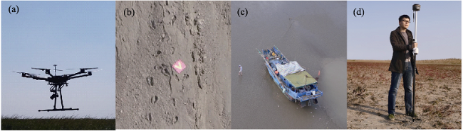
Figure 2 (a) DJI M600 UAV and Zenmuse X5 camera; (b) GCPs; (c) Observation vessel; (d) RTK-GPS
The UAV operation route was set up, which could be seen in Figure 1b. The UAV was operated during the period of ebb tide or half tide, so that it could get more information on the ground. Some weather factors, such as rainfall, snow, hail, and force-5 or higher wind, would not influence the UAV operation. Beside these conditions, the sunlight exposure is the most important factor affecting image quality. So the UAV flight was more suitable to operate in the morning, evening, or cloudy low-light periods of a day. Moreover, when the oblique photogrammetry was been used, the angle of the camera could not switch to the direction of the sunlight. In the present study, the study area consisted of muddy tidal creeks in the Chuandong port area of Jiangsu, and the observation period was July 2018. During the UAV operation, flight height was set to be 80 m with a tilting angle of 45° from different directions.
Figure 1b also showed the location of GCPs and RTK points. Ten colored plastic plates were evenly placed near the tidal creek as the GCPs, and the longitude and latitude coordinates and elevation of the GCPs were measured using the dual-frequency GPS-RTK positioning system based on WGS-85. GCPs provided spatial coordinate information to the UAVs, which was used to accurately control the 3D modelling.
In order to test the accuracy of the DEM and TPF method, RTK-GPS measurement was performed at 185 stations on 16 cross-sections of the tidal creek to obtain the longitude, latitude, and elevation information. Furthermore, 2314 UAV images were taken with a spatial resolution of 2 cm, and the longitudinal and side overlaps of adjacent images were both over 80%.

2.3 Data processing

2.3.1 Structure-from-Motion (SfM)
SfM is an algorithm for 3D reconstruction based on unordered images taken in the study area. With SfM, the 3D spatial coordinates of the study object are determined by changing the position of the camera, to realize the transformation from the two-dimensional (2D) image data to the 3D topographic information (Snavely et al., 2008; Gomez et al., 2015). In the field of computer vision, SfM algorithm has the ability to restore image attitude information and create scene structure information simultaneously. As for the relationship between the UAV and SfM algorithm, the UAV oblique photogrammetry can obtain both top and facade information of the target simultaneously, becoming a bridge connecting the traditional aerial photogrammetry and ground close-range photogrammetry. At present, it is very common to use the UAV images as data source for SfM sparse reconstruction of oblique images (Westoby et al., 2012; Ishiguro et al., 2016; Hayakawa, 2020).
The objective of SfM is to find the same point in the 3D model among multiple images with a high degree of overlap to form stable and accurate stereo pair of feature points. As UAVs have a short operating cycle, the surface of a mudflat can be considered unchanged. Besides, some practices have shown that the clear, shallow water has little influence on the establishment of the 3D model (Dietrich, 2017; Kasvi et al., 2019; Akay et al., 2019). Therefore, the DEM of a tidal flat established by SfM can generate satisfactory results. However, the land-ocean interaction is very strong in a tidal creek, which bears the input and output of plentiful sediment and water. Therefore, it is very difficult for SfM to find invariant feature points among the images, resulting in poor modelling results at the tidal creek. Also, the limitation on UAV flight speed and the short durations of the ebb tide increase the difficulty of data collection.
In this study, the texture features on the photos were more prominent by modifying the contrast of the photos. The SfM processing was done by using Agisoft Photoscan, where you needed manually find the GCPs in all the images, one by one, and tag them.
2.3.2 Trend Prediction Fitting method (TPF)
Just like the introduction saying, UAVs have been successfully used to monitor and acquire the topographic information of tidal flats, but there are few applications to the topographic monitoring of tidal creeks due to water fluctuation. So, the topography of a tidal creek is divided into two parts artificially. The part above the water surface is the exposed topography of the tidal creek, which can be obtained using the SfM method. And the other part needs to be obtained by other methods. In this section, the TPF method is proposed to obtain the underwater topography effectively.
The main principle of the TPF method is shown in Figure 3.
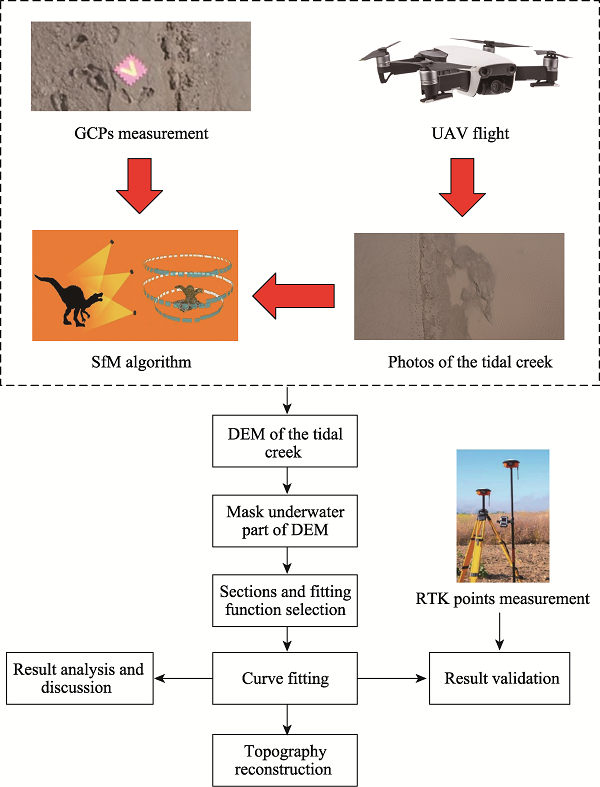
Figure 3 Concept of the TPF method
Under tidal erosion, the tidal creek is high on both sides and low in the middle, with a smooth transition from outside to inside, which generally has good continuity and is very close in shape to the curves of some functions, such as polynomial functions, Gaussian functions, Fourier functions, and sine functions. The elevation of the tidal creek above the water can be monitored with UAVs and SfM algorithm. This elevation can be used to predict the trend of the topography below the water in the middle. A number of cross-sections are selected along the tidal creek, and then the TPF method is used to obtain a new set of cross-sectional topographic information curves. Interpolation is carried out on these curves to eventually obtain the underwater topographic information. Combined with the two parts of above water and underwater a new 3D model of the tidal creek is reconstructed.
In the present study, the polynomial function, Fourier function, Gaussian function, and sum of sine functions were used for curve fitting. Considering the accuracy of the prediction and the amount of calculation, two-order and third-order functions are selected for the fitting prediction, i.e. n=2 and n=3. Higher order functions may be more accurate, but there is less improvement in accuracy for the prediction of bottom elevation.

3 Results

3.1 DEM of the tidal creek generated by SfM only

The DEM of the tidal creek is obtained using the SfM algorithm. The photos taken by the UAV are mainly concentrated in the middle part of the tidal creek, and the DEM is about 600 m long and 200 m wide. As we can see from Figure 4, the elevation of the topography above the water ranges from -1.12 to 2.14 m. Due to the absence of invariant feature points of the fluctuating water, the elevation of the topography below the water surface, as can be clearly seen from the ‘failed part’ in Figure 5, are irregular and very inaccurate. So the underwater topography in Figure 4 is masked manually. Besides, Figure 4 shows the location of RTK points, and we use RTK points in different positions to check the accuracy of DEM. The results of elevation accuracy at the bank and bottom of the tidal creek are shown in Figure 6.
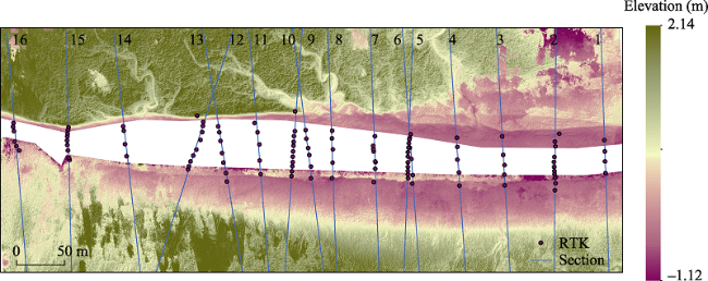
Figure 4 DEM of the tidal creek
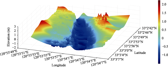
Figure 5 Surface map of the DEM of the tidal creek
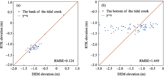
Figure 6 Elevation accuracy at the bank of the tidal creek (a); and Elevation accuracy at the bottom of the tidal creek (b)
In Figure 6a, the RTK points at the bank of the tidal creek have an absolute error of less than 0.3 m, root mean square error (RMSE) of 0.124 m, and mean relative error of 10.9%. The data points have a relatively low degree of dispersion, and the established DEM for the above-water part has relatively high accuracy. In Figure 6b, the RMSE at the RTK points at the bottom of the tidal creek is as high as 1.449 m, indicating that the established DEM for the underwater has low accuracy and this part does not reflect the actual underwater topography.

3.2 Bottom correction by TPF

Based on the distribution of the RTK points, 16 verification cross-sections are selected, which can be seen in Figure 4. The elevation of the topography above the water is extracted from the DEM and preprocessed to eliminate the outliers. Next, the elevation of underwater topography is carried out by TPF method. Considering the range of some functions and for the sake of convenience of calculation and expression, the opposite value of the elevation is used for calculation, fitting, and plotting. The polynomial function, Fourier function, Gaussian function, and sum of sine functions are used separately to perform prediction fitting. Figures 7-10 show the fitting results in each section using each function.
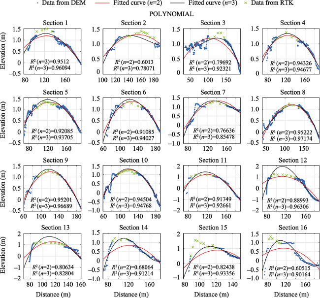
Figure 7 Bottom predictions with polynomial function
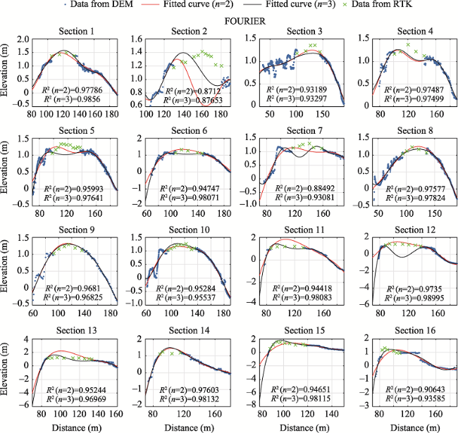
Figure 8 Bottom predictions with Fourier function
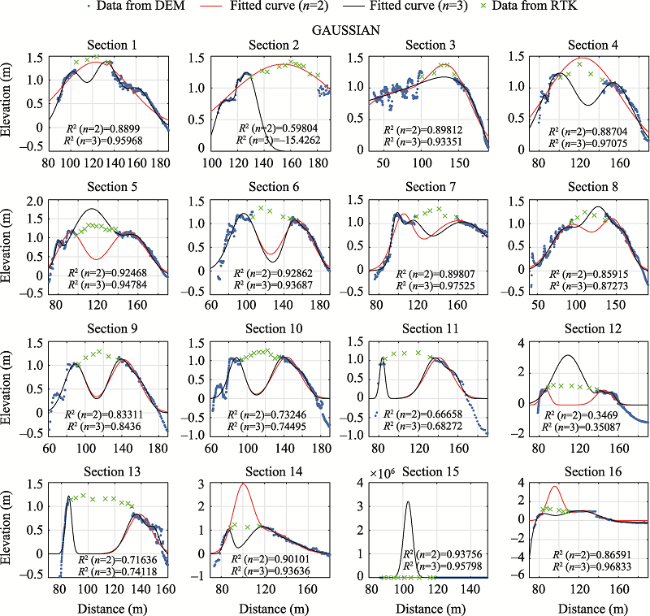
Figure 9 Bottom predictions with Gaussian function
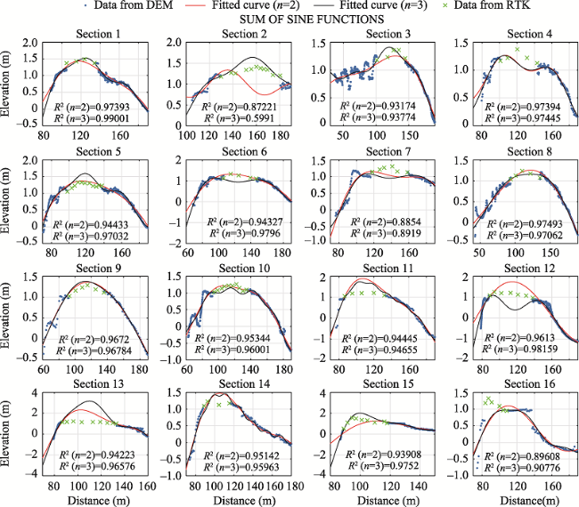
Figure 10 Bottom predictions with sum of sine functions
As can be seen in Figure 7, the second-order and third-order polynomial functions have fine fitting results on most sections, with R2 above 0.8. However, the curves of the second-order polynomial in sections 13-16 are not well matched with DEM points. These sections are characterized by steep slopes on the one side and flat, asymmetrical slopes on the other side. So it is not difficult to imagine that the fitting results of symmetric second-order polynomial function are not good.
As can be seen in Figure 8, the second-order and third-order Fourier functions have good results on most sections, with R2 above 0.9, and only obvious fitting failure appears at section 2. The curves of the second-order Fourier functions is relatively flat, and the third-order Fourier function may have a reverse peak in the middle position, as shown in sections 7 and 12. The reason may be that the steep slope on the left is followed by a gentle slope, and this tends to extend the curve in the opposite direction. In this case, it is much less likely to make an error by using the second-order Fourier functions. For the asymmetrical section shape of sections 13-16, it can be seen that the fitting results of the third-order Fourier function is very good.
In Figure 9, it is easy to see that the Gaussian function is not suitable for the curve fitting, and it fails in many sections, such as sections 2, 6 and 9-16.
As can be seen in Figure 10, the second-order and third-order sum of sine functions have good results on most sections, with R2 above 0.8. However, there is a large error in sections 2, 4, 11 and 12 compared with the RTK points. For the asymmetrical section shape of sections 13-16, the sum of sine functions don't fit very well.

3.3 Evaluation of the TPF method for this tidal creek

In the present study, the polynomial function, Fourier function, Gaussian function, and sum of sine functions are used for prediction fitting at each cross-section. Comparison of the point elevation on the bottom prediction line with the measured RTK point at the corresponding position revealed that in section 15 of Figure 9, the curve fitting is a failure, with an error more than two million meters. This is a rare case, and it is not necessary to put this case in the discussion of error distribution. Figures 11 and 12 show the error distribution for the fitting method with each type of two-order and three-order functions.
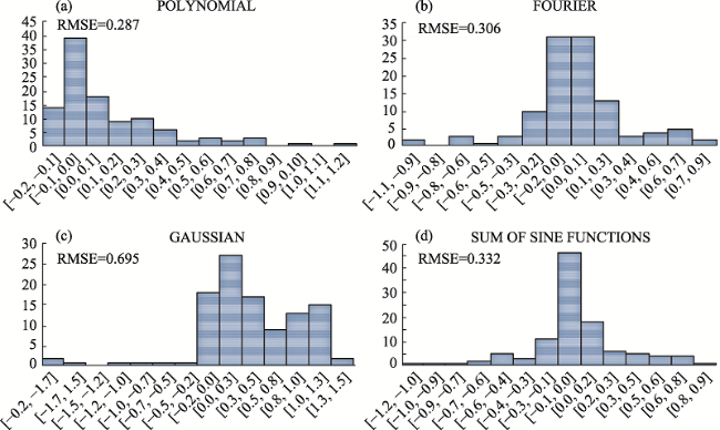
Figure 11 Error distribution with different fit functions (n=2)
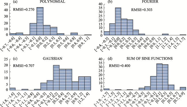
Figure 12 Error distribution with different fit functions (n=3)
The prediction error of the polynomial function is the smallest, and mainly distributed between -0.2 and 0.2 m. RMSE of the two-order polynomial is 0.287 m and RMSE of the three-order is 0.270 m. The prediction error of the Fourier function is small, and mainly distributed between -0.3 and 0.3 m. RMSE of the two-order Fourier is 0.306 m and RMSE of the three-order is 0.303 m. The main distribution of prediction error of the Gaussian function is very disorderly, and RMSE value is above 0.6 m. The prediction error of the sum of sine functions is relatively large, and mainly distributed between -0.3 and 0.3 m, and RMSE of the two-order sum of sine functions is 0.332 m and RMSE of the three-order is 0.400 m.
Overall, the RMSEs for the prediction of the bottom elevation of the tidal creek by the polynomial function and Fourier function are relatively small, while those by the Gaussian function and sum of sine functions are relatively large.
Based on the fitting results and error distribution, the polynomial function and Fourier function are more suitable for the TPF method. So the other 12 sections are selected and TPF method was used for further verification. The positions of the sections are shown in Figure 13 and the fitting results were shown in Figures 14 and 15.
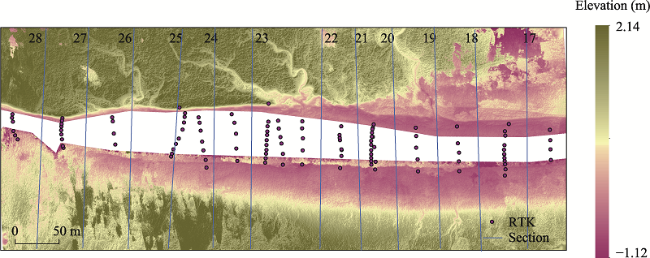
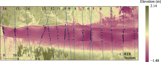
Figure 13 The position of additional 12 sections
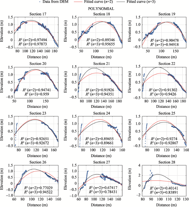
Figure 14 TPF method with polynomial function
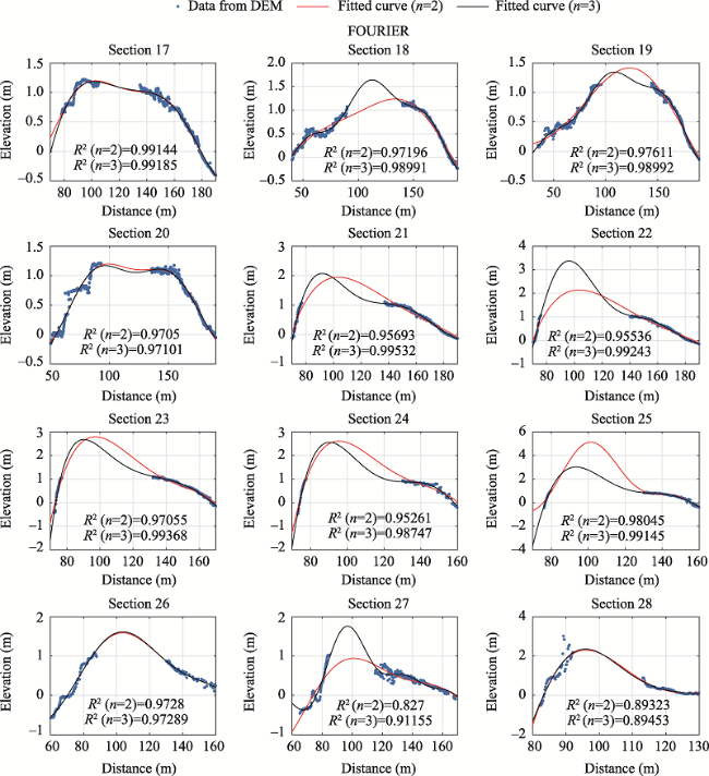
Figure 15 TPF method with Fourier function
As can be seen from Figures 14 and 15, the shape of sections 17-20 is relatively symmetrical. Both polynomial function and Fourier have good fitting curve shape. But the shape of sections 21-28 is a steep slope on one side and a gentle slope on other side. In these sections, the fitting curve of polynomial function does not agree with DEM points on the steep slope side, while the fitting curve of Fourier function has better results. Considering all cross-sections, the well-fitting curves of the polynomial functions and Fourier function are selected to complete the missing underwater topography part. Based on the completed cross-sections, the data points are interpolated and reconstructed using the four-point spline interpolation method in the grid to generate the topographic surface of the tidal creek. The results are shown in Figures 16 and 17. Finally, we obtain a complete 3D morphology of the tidal creek.
Figure 16 DEM of tidal creek corrected by TPF method
Figure 17 Surface map of tidal creek corrected by TPF method

4 Discussion

4.1 Analysis of TPF method

In this study, the polynomial function has linear characteristics and can provide satisfactory results for various forms of topographic cross-sections. It has small RMSE and the best stability. The Fourier function has small RMSE, and is more suitable for the specific tidal creek section. The Gaussian function has the poor fitting curve and the largest RMSE, so it is not suitable for the prediction of the underwater topography. For the case of the sum of sine functions, most checkpoints correspond to errors but reverse peaks are unavoidable. Its RMSEs are larger than RMSEs of the polynomial and Fourier function too. So the polynomial function and the Fourier function have more advantages.
The shape of sections has some influence on the selection of the TPF method. In this study, the research object is a small tidal creek, and it can be found that the shape of sections is mainly divided into two types. The first is the symmetric section, which is relatively simple, and both functions can obtain good fitting results. The second is a steep slope on one side and a gentle slope on the other, in which case the Fourier function gets a better result. In addition, it is noted that when a steep slope is followed by a gentle slope, the three-order Fourier function is prone to show reverse peaks. This phenomenon can be seen from sections 4, 7 and 12 in Figure 8.
Also, whether the selected cross-section is perpendicular to the central axis of the tidal creek there is still some influence on the fitting results. Among the 16 sections in Figure 4 selected in the present study, sections 12 and 13 have relatively large tilting angles with respect to the central axis. Figures 7-10 show that the fitting results for sections 12 and 13 using any of the four functions are not very satisfactory. In addition, for the additional 12 sections in Figure 13, they all try to be perpendicular to the central axis of the tidal creek. Neither the polynomial nor the Fourier fitting curves have any unusual shape.
Finally, the order of the function has some influence on the fitting result. In the present study, two-order and three-order functions are selected for the fitting prediction. As can be seen from Figures 7 and 14, for the polynomial functions, the difference between two-order and three-order curves generally occurs at sections such as sections 12-16 and 27-28. These sections are usually asymmetric and are more suitable for three-order polynomial functions. As can be seen from Figures 8 and 15, for the Fourier function. The two- and three-order curves are in good agreement at most sections. In a few sections, such as sections 12, 22 and 25, there is a great difference. It is suggested that both two-order and three-order Fourier functions should be applied and the curve with a better shape should be selected. It cannot be denied that increasing the order of functions may improve the accuracy of the fitting curve. However, in practice, it is found that the improved accuracy has less improvement in accuracy for the prediction of bottom elevation, and the higher order fitting can lead to the problem of over-fitting. So this study did not investigate the influence of functions above three-order. Meanwhile, the accuracy of the reconstructed area is positively correlated with the number of cross-sections. However, the issue of selecting a suitable number of cross-sections within a particular area under the considerations of the amount of calculations and accuracy has not been considered in the present study and will be investigated in the future.

4.2 Limitation of TPF method

Based on the analysis in the above sections, this part summarizes the limitation of the TPF method. First of all, the TPF method requires some preliminary work, which is mainly related to DEM acquisition of tidal creeks. GCPs are the bridge to transmit information to the 3D point cloud, which is very important to the SFM algorithm. So, it is necessary to lay out GCPs along the tidal creek and measure the latitude, longitude and elevation information. During low tide, Photogrammetry is carried out on the exposed terrain of tidal creek by the UAV. The flight of UAV can also be affected by factors such as weather and the contrast of the photos shot by UAV need to be adjusted. Likewise, when SfM algorithm is used to establish DEM model of the tidal creek, it also needs adjustment and modification for many times.
Secondly, the TPF method is more suitable for tidal creeks with some characteristics. The limitation of SFM algorithm indicates that TPF method is suitable for the tidal creek with clear texture and no vegetation cover, so that the photos obtained can be matched more quickly for feature points, and the DEM established has higher accuracy. Also, due to the limitation of UAV flight speed and short duration of ebb tide, TPF method is more suitable for detecting tidal creeks in small areas. The area of the tidal creek observed in this study is about 1100 m long and 300 m wide. If the length of tidal creeks reaches to thousands of meters, UAV photography may take much longer time. As can be seen from curve-fitting results, the width of the water surface should not be too large, and the sections should be as perpendicular to the central axis of the tidal creek as possible. So the relatively straight tidal creek is easier to meet such requirements.
Finally, there are still some problems that can be further studied. Is it possible to minimize the number of GCPs placed in a particular study area without too much reduction in DEM accuracy? How many sections can be selected in the DEM to control the accuracy of TPF method within an acceptable range? It is helpful to reduce the workload of field observation and quickly obtain the underwater topography of tidal creek.
In a word, the TPF method is carried out on the basis of DEM obtained by SfM algorithm, and is more suitable for small, straight tidal creeks with clear texture and no vegetation cover.

5 Conclusions

In this study, a TPF method is proposed to obtain the underwater topography to form a complete 3D topography of the tidal creek. Based on the images acquired by UAV photogrammetry, the DEM of the tidal creek in the study area has been established by using the SfM technique. The results of verification have shown that the RMSE of the DEM elevation is 12 cm. Some cross-sections have been selected on the DEM of the tidal creek. The TPF method has been carried out by using a polynomial function, Fourier function, Gaussian function, and sum of sine functions. The results have shown that the polynomial function can be adapted to most shape of sections. The Fourier function is more suitable for the asymmetric cross-section with a steep slope on one side and a gentle slope on the other. The Gaussian function leads to very poor results. The sum of sine functions has little advantage over the polynomial function and Fourier function. In the selection of cross-sections, the section should be as perpendicular to the central axis of the tidal creek as possible. The order of the function has a certain influence on the fitting result. Generally, compared with the two-order function, the three-order function lends itself to more complex sections. Meanwhile, the TPF method has some limitations. It needs a lot of preliminary work to get the DEM of the tidal creek. It is more suitable for small, straight tidal creeks with clear texture and no vegetation cover. The technique can be applied to acquire the elevation of tidal creeks precisely, so the more elaborated evolution of tidal creek within one year, one season or even one month could be unveiled only by observational means in the future. In addition, geomorphologist tries to simulate the evolution of tidal creek, but it is not yet simulated very well using hydrodynamic models, as the lack of parameter of water depth. This study could provide water depth data in high frequency.
[1]
Akay S S, Ozcan O, Sen O L, 2019. Modeling morphodynamic processes in a meandering river with unmanned aerial vehicle-based measurements. Journal of Applied Remote Sensing, 13(4): 1-18.

[2]
Allen, J R L, 2000. Morphodynamics of Holocene salt marshes: A review sketch from the Atlantic and Southern North Sea coasts of Europe. Quaternary Science Reviews, 19(12): 1155-1231.

DOI

[3]
Bearman J A, Friedrichs C T, Jaffe B E et al., 2010. Spatial trends in tidal flat shape and associated environmental parameters in South San Francisco Bay. Journal of Coastal Research, 26(2): 342-349.

[4]
Brunier G, Fleury J, Anthony E J et al., 2016. Close-range airborne Structure-from-Motion photogrammetry for high-resolution beach morphometric surveys: Examples from an embayed rotating beach. Geomorphology, 261: 76-88.

DOI

[5]
Chen L C, 1998. Detection of shoreline changes for tideland areas using multi-temporal satellite images. International Journal of Remote Sensing, 19(17): 3383-3397.

DOI

[6]
Coco G, Zhou Z, van Maanen B et al., 2013. Morphodynamics of tidal networks: Advances and challenges. Marine Geology, 346: 1-16.

DOI

[7]
Dai W, Li H, Gong Z et al., 2019. Application of unmanned aerial vehicle technology in geomorphological evolution of tidal flat. Advances in Water Science, 30(3): 359-372. (in Chinese)

[8]
D’Alpaos A, Lanzoni S, Marani M et al., 2005. Tidal network ontogeny: Channel initiation and early development. Journal of Geophysical Research, 110: F02001.

[9]
Dash J, Pearse G, Watt M, 2018. UAV multispectral imagery can complement satellite data for monitoring forest health. Remote Sensing, 10(8): 1216.

DOI

[10]
Davies G, Woodroffe C D, 2010. Tidal estuary width convergence: Theory and form in North Australian estuaries. Earth Surface Processes and Landforms, 35(7): 737-749.

[11]
Dietrich J T, 2017. Bathymetric Structure-from-Motion: Extracting shallow stream bathymetry from multi-view stereo photogrammetry. Earth Surface Processes and Landforms, 42(2): 355-364.

DOI

[12]
Elgar S, Raubenheimer B, 2011. Currents in a small channel on a sandy tidal flat. Continental Shelf Research, 31(1): 9-14.

DOI

[13]
Fagherazzi S, Mariotti G, 2012. Mudflat runnels: Evidence and importance of very shallow flows in intertidal morphodynamics. Geophysical Research Letters, 39(14): L14402.

[14]
Fruergaard M, Andersen T J, Nielsen L H et al., 2011. Punctuated sediment record resulting from channel migration in a shallow sand-dominated micro-tidal lagoon, Northern Wadden Sea, Denmark. Marine Geology, 280: 91-104.

DOI

[15]
Gomez C, Hayakawa Y, Obanawa H, 2015. A study of Japanese landscapes using structure from motion derived DSMs and DEMs based on historical aerial photographs: New opportunities for vegetation monitoring and diachronic geomorphology. Geomorphology, 242: 11-20.

DOI

[16]
Gong Z, Wang Z B, Stive M J F et al., 2012. Process-based morphodynamic modeling of a schematized mudflat dominated by a long-shore tidal current at the Central Jiangsu Coast, China. Journal of Coastal Research, 28(6): 1381-1392.

[17]
Hayakawa Y S, Obanawa H, 2020. Volumetric change detection in bedrock coastal cliffs using terrestrial laser scanning and UAS-based SfM. Sensors, 20(12): 3403.

DOI

[18]
Hibma A, Stive M J F, Wang Z B, 2004. Estuarine morphodynamics. Coastal Engineering, 51: 765-778.

DOI

[19]
Hood W G, 2010. Tidal channel meander formation by depositional rather than erosional processes: Examples from the prograding Skagit River Delta (Washington, USA). Earth Surface Processes and Landforms, 35(3): 319-330.

DOI

[20]
Hughes Z J, 2012. Tidal channels on tidal flats and marshes. In: Richard A Fuller, Robert W Dalrymple eds. Principles of Tidal Sedimentology. Dordrecht, Netherlands: Springer 269-300.

[21]
Ichoku C, Chorowicz J, 1994. A numerical approach to the analysis and classification of channel network patterns. Water Resources Research, 30(2): 161-174.

DOI

[22]
van Iersel W, Straatsma M, Middelkoop H et al., 2018. Multitemporal classification of river floodplain vegetation using time series of UAV images. Remote Sensing, 10(7): 1144.

DOI

[23]
Ishiguro S, Yamano H, Oguma H, 2016. Evaluation of DSMs generated from multi-temporal aerial photographs using emerging structure from motion-multi-view stereo technology. Geomorphology, 268: 64-71.

DOI

[24]
Kasvi E, Salmela J, Lotsari E et al., 2019. Comparison of remote sensing based approaches for mapping bathymetry of shallow, clear water rivers. Geomorphology, 333: 180-197.

DOI

[25]
Lanzoni S, D’Alpaos A, 2015. On funneling of tidal channels. Journal of Geophysical Research: Earth Surface, 120(3): 433-452.

DOI

[26]
Li C X, Z J Q, Fan D et al., 2001. Holocene regression and the tidal radial sand ridge system formation in the Jiangsu coastal zone, East China. Marine Geology, 173: 97-120.

DOI

[27]
Liu Y X, Zhou M X, Zhao S S et al., 2015. Automated extraction of tidal creeks from airborne laser altimetry data. Journal of Hydrology, 527: 1006-1020.

DOI

[28]
Magolan, J L, Halls J N, 2020. A multi-decadal investigation of tidal creek wetland changes, water level rise, and ghost forests. Remote Sensing, 12(7): 1141.

DOI

[29]
Mallin M A, Lewitus A J, 2004. The importance of tidal creek ecosystems. Journal of Experimental Marine Biology and Ecology, 298(2): 145-149.

DOI

[30]
Mancini F, Dubbini M, Gattelli M et al., 2013. Using unmanned aerial vehicles (UAV) for high-resolution reconstruction of topography: The structure from motion approach on coastal environments. Remote Sensing, 5(12): 6880-6898.

DOI

[31]
Mariotti G, Fagherazzi S, 2012. Channels-tidal flat sediment exchange: The channel spillover mechanism. Journal of Geophysical Research: Oceans, 117: C03032.

[32]
Mason D C, Davenport I J, Flather R A, 1997. Interpolation of an intertidal digital elevation model from heighted shorelines: A case study in the Western Wash. Estuarine, Coastal and Shelf Science, 45(5): 599-612.

DOI

[33]
Mason D C, Davenport I J, Flather R A et al., 1998. A digital elevation model of the inter-tidal areas of the Wash, England, produced by the waterline method. International Journal of Remote Sensing, 19(8): 1455-1460.

DOI

[34]
Mason D C, Scott T R, H-J Wang. 2006. Extraction of tidal channel networks from airborne scanning laser altimetry. ISPRS Journal of Photogrammetry & Remote Sensing, 61: 67-83.

[35]
Meinen B U, Robinson D T, 2020. Mapping erosion and deposition in an agricultural landscape: Optimization of UAV image acquisition schemes for SfM-MVS. Remote Sensing of Environment, 239: 111666.

DOI

[36]
Mohamad N, Abdul Khanan M F, Ahmad A et al., 2019. Evaluating water level changes at different tidal phases using UAV photogrammetry and GNSS vertical data. Sensors, 19(17): 3778.

DOI

[37]
d’Oleire-Oltmanns S, Marzolff I, Peter K et al., 2012. Unmanned aerial vehicle (UAV) for monitoring soil erosion in Morocco. Remote Sensing, 4(11): 3390-3416.

DOI

[38]
Perillo G M E, 2009. Tidal courses: Classification, origin and functionality. In: Coastal Wetlands: An Integrated Ecosystem Approach. New York: Elsevier Science, 185-209.

[39]
Rao W B, Mao C P, Wang Y G et al., 2015. Geochemical constraints on the provenance of surface sediments of radial sand ridges off the Jiangsu coastal zone, East China. Marine Geology, 359: 35-49.

DOI

[40]
Shi B W, Cooper J R, Pratolongo P D et al., 2017. Erosion and accretion on a mudflat: The importance of very shallow‐water effects. Journal of Geophysical Research: Oceans, 122(12): 9476-9499.

DOI

[41]
Snavely N, Seitz S M, Szeliski R, 2008. Modeling the world from internet photo collections. International Journal of Computer Vision, 80(2): 189-210.

DOI

[42]
Stefanon L, Carniello L, D’Alpaos A et al., 2012. Signatures of sea level changes on tidal geomorphology: Experiments on network incision and retreat. Geophysical Research Letters, 39: L12402.

[43]
Stevenson J A, Sun X F, Mitchell N C, 2010. Despeckling SRTM and other topographic data with a denoising algorithm. Geomorphology, 114: 238-252.

DOI

[44]
Tong X H, Liu X F, Chen P et al., 2015. Integration of UAV-based photogrammetry and terrestrial laser scanning for the three-dimensional mapping and monitoring of open-pit mine areas. Remote Sensing, 7(6): 6635-6662.

DOI

[45]
Um I, Park S, Kim H T et al., 2020. Configuring RTK-GPS architecture for system redundancy in multi-drone operations. IEEE Access, 8: 76228-76242.

DOI

[46]
Vandenbruwaene W, Meire P, Temmerman S, 2012. Formation and evolution of a tidal channel network within a constructed tidal marsh. Geomorphology, 151/152: 114-125.

DOI

[47]
Vlaswinkel B M, Cantelli A, 2011. Geometric characteristics and evolution of a tidal channel network in experimental setting. Earth Surface Processes and Landforms, 36: 739-752.

DOI

[48]
Wang X Y, Ke X K, 1997. Grain-size characteristics of the extant tidal flat sediments along the Jiangsu coast, China. Sedimentary Geology, 112: 105-122.

DOI

[49]
Wang Y, Zhu D K, You K Y et al., 1999. Evolution of radiative sand ridge field of the South Yellow Sea and its sedimentary characteristics. Science in China Series D Earth Sciences, 42: 97-112.

[50]
Wang, Y P, Gao S, Jia J J et al., 2012. Sediment transport over an accretional intertidal flat with influences of reclamation, Jiangsu coast, China. Marine Geology, 291- 294: 147-161.

[51]
Watts A C, Ambrosia V G, Hinkley E A, 2012. Unmanned aircraft systems in remote sensing and scientific research: Classification and considerations of use. Remote Sensing, 4(6): 1671-1692.

DOI

[52]
Westoby M J, Alfieri J, Glasser N F et al., 2012. ‘Structure-from-Motion’ photogrammetry: A low-cost, effective tool for geoscience applications. Geomorphology, 179: 300-314.

DOI

[53]
Xing F, Wang Y P, Wang H V, 2012. Tidal hydrodynamics and fine-grained sediment transport on the radial sand ridge system in the southern Yellow Sea. Marine Geology, 291-294: 192-210.

DOI

[54]
Yin Y H, 1997. Actuality and advances in tidal creeks. Marine Geology Letters, 1-4. (in Chinese)

[55]
Zhang C K, Xu M P, Zhou Z et al., 2018. Advances in cross-shore profile characteristics and sediment sorting dynamics of tidal flats. Advances in Water Science, 29(2): 269-282. (in Chinese)

[56]
Zhang R S, 1992. Suspended sediment transport processes on tidal mud flat in Jiangsu Province, China. Estuarine, Coastal and Shelf Science, 35(3): 225-233.

DOI

[57]
Zhang S M, Zhao G X, 2019. A harmonious satellite-unmanned aerial vehicle-ground measurement inversion method for monitoring salinity in coastal saline soil. Remote Sensing, 11(14): 1700.

DOI

[58]
Zhao B X, Liu Y X, Xu W X et al., 2019. Morphological characteristics of tidal creeks in the central coastal region of Jiangsu, China, using LiDAR. Remote Sensing, 11(20): 2426.

DOI

[59]
Zhou Z, Stefanon L, Olabarrieta M et al., 2014. Analysis of the drainage density of experimental and modelled tidal networks. Earth Surface Dynamics, 2: 105-116.

DOI

Outlines

/