
Journal of Geographical Sciences >
Impacts of traffic accessibility on ecosystem services: An integrated spatial approach
|
Chen Wanxu (1989-), PhD, specialized in resource and environment assessment and regional economic analysis. E-mail: cugcwx@cug.edu.cn |
Received date: 2020-10-07
Accepted date: 2021-03-10
Online published: 2022-02-25
Supported by
National Natural Science Foundation of China(42001187)
National Natural Science Foundation of China(41701629)
Copyright
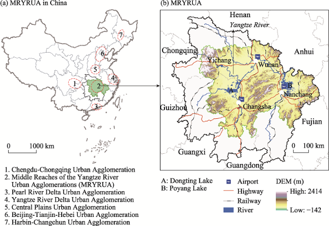
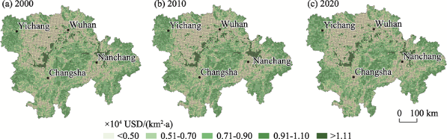
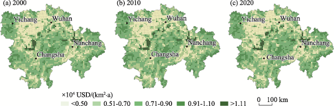
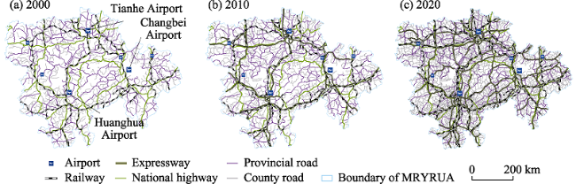
The continuous degradation of ecosystem services is an important challenge faced by the world. Improvements in transportation infrastructure have had substantial impacts on economic development and ecosystem services. Exploring the influence of traffic accessibility on ecosystem services can delay or stop their deterioration; however, studies on its impact are lacking. This study addresses this gap by analysing the impact of traffic accessibility on ecosystem services using an integrated spatial regression approach based on an evaluation of the ecosystem services value (ESV) and traffic accessibility in the Middle Reaches of the Yangtze River Urban Agglomeration (MRYRUA) in China. The results indicated that the ESV in the MRYRUA continuously decreased during the study period, and the average ESV in plain areas, areas surrounding the core cities, and areas along the main traffic routes was significantly lower than that in areas along the Yangtze River and the surrounding mountainous areas. Traffic accessibility continued to increase during the study period, and the high-value areas centred on Wuhan, Changsha, Nanchang, and Yichang were radially distributed. The global bivariate spatial autocorrelation coefficient between the average ESV and traffic accessibility was negative. The average ESV and traffic accessibility exhibited significant spatial dependence and spatial heterogeneity. Spatial regression also proved that there was a negative association between the average ESV and traffic accessibility, and scale effects were evident. The findings of this study have important policy implications for future ecological protection and transportation planning.
CHEN Wanxu , ZENG Yuanyuan , ZENG Jie . Impacts of traffic accessibility on ecosystem services: An integrated spatial approach[J]. Journal of Geographical Sciences, 2021 , 31(12) : 1816 -1836 . DOI: 10.1007/s11442-021-1924-y
Figure 1 Location of the study area (Middle Reaches of the Yangtze River Urban Agglomeration) in China |
Table 1 Evaluation criteria for each index for traffic accessibility |
| Type | Sub-type | Level | Standard | Score |
|---|---|---|---|---|
| Railway | - | 1 | Owning railway | 2 |
| 2 | 30 km from the railway | 1.5 | ||
| 3 | 60 km from the railway | 1 | ||
| 4 | Others | 0 | ||
| Road | Expressway | 1 | Owning expressway | 1.5 |
| 2 | 30 km from the expressway | 1 | ||
| 3 | 30 km from the expressway | 0.5 | ||
| 4 | Others | 0 | ||
| National road | 1 | Owning national road | 0.5 | |
| 2 | Others | 0 | ||
| Provincial road | 1 | Owning provincial road | 0.3 | |
| 2 | Others | 0 | ||
| County road | 1 | Owning county road | 0.1 | |
| 2 | Others | 0 | ||
| Shipping transport | Hub ports | 1 | Owning hub ports | 1.5 |
| 2 | 30 km from the hub ports | 1 | ||
| 3 | 30 km from the hub ports | 0.5 | ||
| 4 | Others | 0 | ||
| General ports | 1 | Owning general ports | 0.5 | |
| 2 | Others | 0 | ||
| Airports | International airports | 1 | Owning international airports | 1 |
| 2 | 30 km from international airports | 0.5 | ||
| 3 | Others | 0 | ||
| General airports | 1 | Owning general airports | 0.5 | |
| 2 | Others | 0 | ||
| Central cities | - | 1 | 100 km from city centres | 2 |
| 2 | 300 km from central cities | 1.5 | ||
| 3 | 600 km from central cities | 1 | ||
| 4 | Others | 0 | ||
| Density of navigable river (m/km2) | - | 1 | >600 | 2 |
| 2 | (200, 600] | 1.5 | ||
| 3 | (0, 200] | 1 | ||
| 4 | 0 | 0 | ||
| Railway density (m/km2) | - | 1 | >300 | 2 |
| 2 | (100, 300] | 1.5 | ||
| 3 | (0, 100] | 1 | ||
| 4 | 0 | 0 | ||
| Road density (m/km2) | - | 1 | >1500 | 2 |
| 2 | (1000, 1500] | 1.5 | ||
| 3 | (0, 1000] | 1 | ||
| 4 | 0 | 0 |
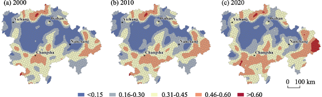
Figure 2 Spatial distribution of average ESV at the 5-km grid scale in the Middle Reaches of the Yangtze River Urban Agglomeration |
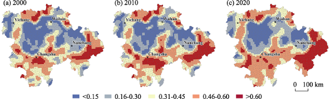
Figure 3 Spatial distribution of average ESV at the 10-km grid scale in the Middle Reaches of the Yangtze River Urban Agglomeration |
Figure 4 Spatial distribution of traffic network in the Middle Reaches of the Yangtze River Urban Agglomeration |
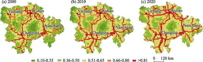
Figure 5 Spatial distribution of traffic accessibility at the 5-km grid scale in the Middle Reaches of the Yangtze River Urban Agglomeration |
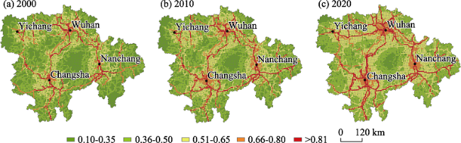
Figure 6 Spatial distribution of traffic accessibility at the 10-km grid scale in the Middle Reaches of the Yangtze River Urban Agglomeration |
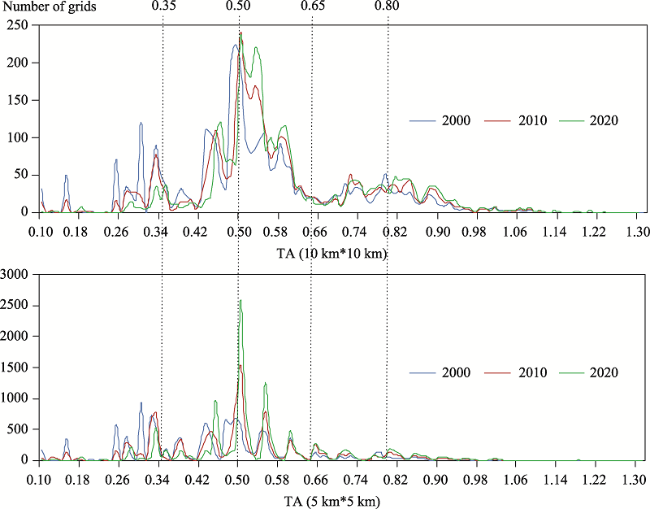
Figure 7 Statistics of traffic accessibility distribution at different scales in the Middle Reaches of the Yangtze River Urban Agglomeration |
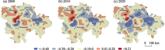
Figure 8 Bivariate LISA cluster maps between average ecosystem services value and traffic accessibility at the 5-km grid scale in the Middle Reaches of the Yangtze River Urban Agglomeration |
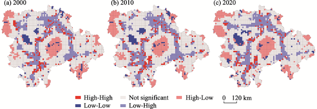
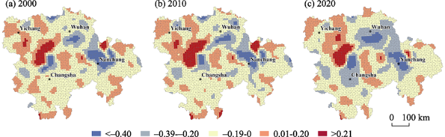
Figure 9 Bivariate LISA cluster maps between average ecosystem services value and traffic accessibility at the 10-km grid scale in the Middle Reaches of the Yangtze River Urban Agglomeration |
Table 2 Regression results of the ordinary least squares (OLS) in the Middle Reaches of the Yangtze River Urban Agglomeration |
| Variables | 5-km grid scale | 10-km grid scale | ||||
|---|---|---|---|---|---|---|
| 2000 | 2010 | 2020 | 2000 | 2010 | 2020 | |
| TA | ‒0.146*** (0.010) | ‒0.159*** (0.010) | ‒0.261*** (0.011) | ‒0.141*** (0.016) | ‒0.135*** (0.017) | ‒0.201*** (0.017) |
| Population density | ‒0.631*** (0.034) | ‒0.796*** (0.038) | ‒0.907*** (0.040) | ‒0.419*** (0.052) | ‒0.556*** (0.056) | ‒0.640*** (0.058) |
| Elevation | 0.253*** (0.009) | 0.246*** (0.009) | 0.246*** (0.009) | 0.215*** (0.014) | 0.218*** (0.015) | 0.225*** (0.014) |
| Constant | 0.406*** (0.004) | 0.416*** (0.005) | 0.458*** (0.005) | 0.424*** (0.008) | 0.427*** (0.009) | 0.450*** (0.009) |
| Moran’s I (error) | 0.595*** | 0.592*** | 0.574*** | 0.558*** | 0.554*** | 0.542*** |
| LM (lag) | 16202.969*** | 15949.124*** | 14942.003*** | 3400.421*** | 3336.905*** | 3166.978*** |
| Robust LM (lag) | 52.994*** | 49.676*** | 113.351*** | 10.196** | 8.458** | 16.859*** |
| LM (error) | 16959.133*** | 16805.582*** | 15795.762*** | 3687.966*** | 3630.687*** | 3482.858*** |
| Robust LM (error) | 809.158*** | 906.134*** | 967.110*** | 297.741*** | 302.234*** | 332.738*** |
| LM (lag and error) | 17012.127*** | 16855.258*** | 15909.113*** | 3698.1625*** | 3639.145*** | 3499.716*** |
| Measures of fit | ||||||
| Log likelihood | 8381.890 | 8219.170 | 7834.050 | 2690.940 | 2630.150 | 2583.130 |
| AIC | ‒16755.800 | ‒16430.300 | ‒15660.100 | ‒5373.880 | ‒5252.300 | ‒5158.250 |
| SC | ‒16726.000 | ‒16400.500 | ‒15630.300 | ‒5349.480 | ‒5227.900 | ‒5133.850 |
| R-squared | 0.167 | 0.175 | 0.208 | 0.205 | 0.206 | 0.243 |
| N | 12710 | 12710 | 12710 | 3299 | 3299 | 3299 |
Notes: The study uses the Queen’s contiguity weight matrix. ***p≤0.001, **p≤0.01, *p≤0.05. Standard errors are in parentheses. LM = Lagrange multiplier, AIC = Akaike information criterion, SC = Schwarz criterion. |
Table 3 Regression results of the spatial lag model (SLM) and spatial error model (SEM) at the 5-km grid scale in 2000, 2010, and 2020 in the Middle Reaches of the Yangtze River Urban Agglomeration |
| Variables | 2000 | 2010 | 2020 | |||
|---|---|---|---|---|---|---|
| SLM | SEM | SLM | SEM | SLM | SEM | |
| TA | ‒0.043*** (0.006) | ‒0.059*** (0.008) | ‒0.054*** (0.008) | ‒0.077*** (0.009) | ‒0.075*** (0.008) | ‒0.097*** (0.010) |
| Population density | ‒0.351*** (0.022) | ‒0.561*** (0.029) | ‒0.423*** (0.024) | ‒0.698*** (0.033) | ‒0.473*** (0.027) | ‒0.775*** (0.037) |
| Elevation | 0.042*** (0.006) | 0.223*** (0.016) | 0.038*** (0.006) | 0.217*** (0.016) | 0.044*** (0.006) | 0.248*** (0.017) |
| Spatial lag term | 0.841*** (0.006) | 0.838*** (0.006) | 0.830*** (0.006) | |||
| Spatial error term | 0.858*** (0.006) | 0.856*** (0.006) | 0.852*** (0.006) | |||
| Constant | 0.075*** (0.004) | 0.379*** (0.006) | 0.082*** (0.004) | 0.389*** (0.006) | 0.094*** (0.004) | 0.389*** (0.007) |
| Measures of fit | ||||||
| Log likelihood | 13220.600 | 13308.526 | 12999.600 | 13097.571 | 12420.100 | 12497.926 |
| AIC | ‒26431.100 | ‒26609.100 | ‒25989.200 | ‒26187.100 | ‒24830.200 | ‒24987.900 |
| SC | ‒26393.900 | ‒26579.300 | ‒25951.900 | ‒26157.300 | ‒24792.900 | ‒24958.100 |
| R-squared | 0.664 | 0.671 | 0.663 | 0.671 | 0.665 | 0.673 |
| N | 12710 | 12710 | 12710 | 12710 | 12710 | 12710 |
Notes: The study uses the Queen’s contiguity weight matrix. ***p≤0.001, **p≤0.01, *p≤0.05. Standard errors are in parentheses. LM = Lagrange multiplier, AIC = Akaike information criterion, SC = Schwarz criterion. |
Table 4 Regression results of the spatial lag model (SLM) and spatial error model (SEM) at the 10-km grid scale in 2000, 2010, and 2020 in the Middle Reaches of the Yangtze River Urban Agglomeration |
| Variables | 2000 | 2010 | 2020 | |||
|---|---|---|---|---|---|---|
| SLM | SEM | SLM | SEM | SLM | SEM | |
| TA | ‒0.060*** (0.011) | ‒0.094*** (0.013) | ‒0.060*** (0.012) | ‒0.097*** (0.014) | ‒0.078*** (0.012) | ‒0.120*** (0.015) |
| Population density | ‒0.277*** (0.035) | ‒0.353*** (0.039) | ‒0.367*** (0.037) | ‒0.465*** (0.043) | ‒0.431*** (0.040) | ‒0.553*** (0.046) |
| Elevation | 0.037*** (0.010) | 0.181*** (0.022) | 0.037*** (0.010) | 0.183*** (0.023) | 0.043*** (0.010) | 0.201*** (0.023) |
| Spatial lag term | 0.822*** (0.012) | 0.820*** (0.012) | 0.814*** (0.012) | |||
| Spatial error term | 0.850*** (0.011) | 0.848*** (0.012) | 0.848*** (0.012) | |||
| Constant | 0.096*** (0.007) | 0.409*** (0.011) | 0.099*** (0.008) | 0.414*** (0.011) | 0.109*** (0.008) | 0.414*** (0.012) |
| Measures of fit | ||||||
| Log likelihood | 3806.200 | 3850.878 | 3728.190 | 3772.807 | 3654.160 | 3697.945 |
| AIC | ‒7602.410 | ‒7693.760 | ‒7446.370 | ‒7537.610 | ‒7298.310 | ‒7387.890 |
| SC | ‒7571.900 | ‒7669.350 | ‒7415.870 | ‒7513.210 | ‒7267.810 | ‒7363.490 |
| R-squared | 0.648 | 0.663 | 0.645 | 0.660 | 0.655 | 0.670 |
| N | 3299 | 3299 | 3299 | 3299 | 3299 | 3299 |
Notes: The study uses the Queen’s contiguity weight matrix. ***p≤0.001, **p≤0.01, *p≤0.05. Standard errors are in parentheses. LM = Lagrange multiplier. AIC = Akaike information criterion. SC = Schwarz criterion. |
Figure 10 Results of geographically weighted regression at the 5-km grid scale in the Middle Reaches of the Yangtze River Urban Agglomeration |
Figure 11 Results of geographically weighted regression at the 10-km grid scale in the Middle Reaches of the Yangtze River Urban Agglomeration |
Figure S1 Local R2 of GWR model at the 5-km grid scale in the Middle Reaches of the Yangtze River Urban Agglomeration |
Figure S2 Local R2 of GWR model at the 10-km grid scale in the Middle Reaches of the Yangtze River Urban Agglomeration |
Table S1 The equivalent value per unit area of ecosystem services in the Middle Reaches of the Yangtze River Urban Agglomeration [USD/(ha2·a)] |
| Sub-type | Cultivated land | Forestland | Grassland | Water body | Construction land | Unused land | Wetland |
|---|---|---|---|---|---|---|---|
| Food production | 344.927 | 113.826 | 148.319 | 182.811 | 3.449 | 6.899 | 124.174 |
| Raw materials | 134.522 | 1027.883 | 124.174 | 120.725 | 0.000 | 13.797 | 82.783 |
| Gas regulation | 248.348 | 1490.086 | 517.391 | 175.913 | -834.724 | 20.696 | 831.275 |
| Climate regulation | 334.580 | 1403.854 | 538.087 | 710.550 | 0.000 | 44.841 | 4673.765 |
| Hydrology regulation | 265.594 | 1410.753 | 524.290 | 6474.286 | -2590.404 | 24.145 | 4635.823 |
| Waste treatment | 479.449 | 593.275 | 455.304 | 5122.171 | -848.521 | 89.681 | 4966.953 |
| Soil conservation | 507.043 | 1386.608 | 772.637 | 141.420 | 6.899 | 58.638 | 686.405 |
| Biodiversity maintenance | 351.826 | 1555.622 | 645.014 | 1183.101 | 117.275 | 137.971 | 1272.782 |
| Aesthetic landscape provision | 58.638 | 717.449 | 300.087 | 1531.477 | 3.449 | 82.783 | 1617.709 |
| In total | 2724.926 | 9699.356 | 4025.302 | 15642.454 | -4142.577 | 479.449 | 18891.670 |
Notes: 100 US dollars could be exchanged for 622.84 yuan in 2015. |
Table S2 ESV provided by different land use types in the Middle Reaches of the Yangtze River Urban Agglomeration |
| Years | Cultivated land | Forestland | Grassland | Water body | Wetland | Unused land | Construction land |
|---|---|---|---|---|---|---|---|
| 2000 (×104 USD) | 31791.713 | 145005.741 | 2850.153 | 27040.381 | 10188.576 | 1.305 | -3191.266 |
| 2010 (×104 USD) | 31293.248 | 144899.336 | 2726.990 | 27506.025 | 10967.188 | 1.336 | -3826.940 |
| 2020 (×104 USD) | 30486.233 | 143298.548 | 2673.709 | 27029.617 | 11663.780 | 1.757 | -5762.117 |
| 2000 (%) | 14.878 | 67.859 | 1.334 | 12.654 | 4.768 | 0.001 | -1.493 |
| 2010 (%) | 14.653 | 67.847 | 1.277 | 12.879 | 5.135 | 0.001 | -1.792 |
| 2020 (%) | 14.559 | 68.436 | 1.277 | 12.909 | 5.570 | 0.001 | -2.752 |
| 2000-2010 (%) | -0.225 | -0.012 | -0.057 | 0.225 | 0.367 | 0.000 | -0.298 |
| 2010-2020 (%) | -0.093 | 0.589 | 0.000 | 0.029 | 0.435 | 0.000 | -0.960 |
Table S3 Changes in the structure of ESV in the Middle Reaches of the Yangtze River Urban Agglomeration |
| Type | Sub-type | 2000 (×104) (USD) | 2010 (×104) (USD) | 2020 (×104) (USD) | 2000-2010 (%) | 2010-2020 (%) | 2000-2020 (%) |
|---|---|---|---|---|---|---|---|
| Supplying services | Food production | 6216.652 | 6158.857 | 6036.583 | -0.930 | -1.985 | -2.897 |
| Raw materials | 17277.657 | 17244.980 | 17033.242 | -0.189 | -1.228 | -1.415 | |
| Regulating services | Gas regulation | 25650.091 | 25483.895 | 24792.947 | -0.648 | -2.711 | -3.342 |
| Climate regulation | 29021.262 | 29141.976 | 28954.806 | 0.416 | -0.642 | -0.229 | |
| Hydrology regulation | 36257.218 | 36163.411 | 34608.668 | -0.259 | -4.299 | -4.547 | |
| Waste treatment | 25665.391 | 25784.236 | 25169.144 | 0.463 | -2.386 | -1.934 | |
| Supporting services | Soil conservation | 27812.715 | 27714.673 | 27349.710 | -0.353 | -1.317 | -1.665 |
| Biodiversity maintenance | 30640.394 | 30644.914 | 30341.243 | 0.015 | -0.991 | -0.976 | |
| Cultural services | Aesthetic landscape provision | 15145.224 | 15230.242 | 15105.186 | 0.561 | -0.821 | -0.264 |
| In total | 213686.603 | 213567.183 | 209391.528 | -0.056 | -1.955 | -2.010 | |
| [1] |
|
| [2] |
|
| [3] |
|
| [4] |
|
| [5] |
Modern spatial econometrics in practice: A guide to GeoDa. GeoDa Space and PySAL.
|
| [6] |
|
| [7] |
|
| [8] |
|
| [9] |
|
| [10] |
|
| [11] |
|
| [12] |
|
| [13] |
|
| [14] |
|
| [15] |
|
| [16] |
|
| [17] |
|
| [18] |
|
| [19] |
|
| [20] |
|
| [21] |
|
| [22] |
|
| [23] |
|
| [24] |
|
| [25] |
|
| [26] |
|
| [27] |
|
| [28] |
|
| [29] |
|
| [30] |
|
| [31] |
|
| [32] |
|
| [33] |
|
| [34] |
|
| [35] |
|
| [36] |
|
| [37] |
|
| [38] |
|
| [39] |
|
| [40] |
|
| [41] |
|
| [42] |
Millennium Ecosystem Assessment (MEA), 2005. Ecosystems and Human Well-being. Washington, DC: Island Press.
|
| [43] |
|
| [44] |
|
| [45] |
|
| [46] |
|
| [47] |
|
| [48] |
|
| [49] |
|
| [50] |
|
| [51] |
|
| [52] |
|
| [53] |
|
| [54] |
|
| [55] |
|
| [56] |
|
| [57] |
|
| [58] |
|
| [59] |
|
| [60] |
|
| [61] |
|
| [62] |
|
| [63] |
|
/
| 〈 |
|
〉 |
