Research Articles

Three-dimensional modelling of soil organic carbon density and carbon sequestration potential estimation in a dryland farming region of China

  • SUN Zhongxiang , 1 ,
  • BAI Huiqing 2 ,
  • YE Huichun 1, 3 ,
  • ZHUO Zhiqing 4 ,
  • HUANG Wenjiang , 1, 3, 5, *
Expand
  • 1. State Key Laboratory of Remote Sensing Science, Aerospace Information Research Institute, CAS, Beijing 100094, China
  • 2. Key Laboratory of Plant Resources, Institute of Botany, CAS, Beijing 100093, China
  • 3. Key Laboratory of Earth Observation of Hainan Province, Sanya 572029, Hainan, China
  • 4. Institute of Agricultural Remote Sensing and Institute of Agricultural Remote Sensing and Information Technology Application, Zhejiang University, Hangzhou 310058, China
  • 5. University of Chinese Academy of Sciences, Beijing 100049, China
*Huang Wenjiang, E-mail:

Sun Zhongxiang (1991-), PhD, specialized in soil organic carbon and spatial analysis. E-mail:

Received date: 2020-12-28

  Accepted date: 2021-07-21

  Online published: 2021-12-25

Supported by

Youth Innovation Promotion Association CAS(2021119)

Future Star Talent Program of Aerospace Information Research Institute, Chinese Academy of Sciences(2020KTYWLZX08)

National Special Support Program for High-level Personnel Recruitment

Abstract

Soil organic carbon density (SOCD) and soil organic carbon sequestration potential (SOCP) play an important role in carbon cycle and mitigation of greenhouse gas emissions. However, the majority of studies focused on a two-dimensional scale, especially lacking of field measured data. We employed the interpolation method with gradient plane nodal function (GPNF) and Shepard (SPD) across a range of parameters to simulate SOCD with a 40 cm soil layer depth in a dryland farming region (DFR) of China. The SOCP was estimated using a carbon saturation model. Results demonstrated the GPNF method was proved to be more effective in simulating the spatial distribution of SOCD at the vertical magnification multiple and search point values of 3.0×10⁶ and 25, respectively. The soil organic carbon storage (SOCS) of 40 cm and 20 cm soil layers were estimated as 22.28×10¹¹ kg and 13.12×10¹¹ kg simulated by GPNF method in DFR. The SOCP was estimated as 0.95×10¹¹ kg considered as a carbon sink at the 20-40 cm soil layer. Furthermore, the SOCP was estimated as -2.49×10¹¹ kg considered as a carbon source at the 0-20 cm soil layer. This research has important values for the scientific use of soil resources and the mitigation of greenhouse gas emissions.

Cite this article

SUN Zhongxiang , BAI Huiqing , YE Huichun , ZHUO Zhiqing , HUANG Wenjiang . Three-dimensional modelling of soil organic carbon density and carbon sequestration potential estimation in a dryland farming region of China[J]. Journal of Geographical Sciences, 2021 , 31(10) : 1453 -1468 . DOI: 10.1007/s11442-021-1906-0

1 Introduction

With climate warming on the rise, international scholars are continuously finding out an effective strategy to control climate change. Increasing carbon sequestration of terrestrial ecosystem can effectively reduce CO2 concentration in the air (Fang et al., 2015). The soil organic carbon (SOC) pool is not only the largest carbon pool in the global terrestrial ecosystem (approximately 1550 Gt) but also twice carbon stored compared with the entire global vegetation. Therefore, SOC is crucial for the global carbon balance (Lal, 2004; Schmidt et al., 2011; Alidoust et al., 2018). Furthermore, SOC also plays a central role in the determination of soil quality (Berg et al., 1993; West et al., 2004; Singh et al., 2007; Singh et al., 2020).
Despite the extensive research conducted on the spatial variation of SOC, most of the studies focused on a two-dimensional (2D) scale, however, these studies only considered the horizontal or vertical direction without any interrelation between the upper and lower soil layers. Actually, soil is a three-dimensional (3D) natural space entity, including both water and nutrients exhibit spatial variability in the horizontal and vertical directions. The spatial variation of SOC has been widely investigated with the application of three-dimensional statistical methods (Castrignanò et al., 2002; Van Meirvenne et al., 2003; Chen et al., 2015). However, as the SOC fails to meet the assumption of second-order stability in the vertical direction, some three-dimensional interpolation methods cannot be directly used to estimate SOC. Previous research has combined the section depth distribution equation with a two-dimensional interpolation method to solve this problem. For example, on a regional scale, negative index equations have been integrated with neural network techniques and two-dimensional Kriging in order to describe SOC and estimate soil organic carbon storage (SOCS) under different depths (Minasny et al., 2006; Malone et al., 2009; Mishra et al., 2009). Chen et al. (2015) and Wang et al. (2020) combined the SOC profile distribution function with three-dimensional Kriging to estimate the SOC. On a landscape scale, Liu et al. (2013) and Lacoste et al. (2014) performed three-dimensional simulations of SOC by fusing the spline functions with both support vector machine and decision tree regression methods. On a farmland scale, Veronesi et al. (2012) integrated polynomial function with a two-dimensional Kriging for three-dimensional simulations of soil firmness. However, these methods are computationally expensive.
The SOC datasets typically used for studies of global carbon cycle can only repreasent a percentage of the SOC content and are thus not able to represent the quality of organic carbon. The SOCD refers to the soil organic carbon reserves in the soil layer at a certain depth under a unit area and can better reflect the variations in the SOCS compared to commonly used datasets (Kumar et al., 2013; Sun et al., 2019). Agriculture has a profound influence on SOCD. Furthermore, the impact of anthropogenic activities on farmland ecosystems has substantially altered the spatial and temporal distribution of SOCD. Thus, a simple and effective strategy must be determined in order to improve the applicability of three-dimensional simulations on SOCD.
The SOC sequestration refers to the transfer of CO2 from the atmosphere into the SOC pool for safe storage. However, the carbon holding capacity of soil is limited by both the carbon input and the stabilization mechanisms of soil organic matter (Six et al., 2002). Numerous studies have proposed and evaluated the concept of soil carbon saturation (Stewart et al., 2008; Du et al., 2014; Waqas et al., 2020). For example, results from long-term field experiments in Africa, Asia, Australia, Europe, and America have demonstrated the presence of SOC saturation, with minimal variations in the SOC content once SOC saturation is reached (Grant et al., 2001; Bayer et al., 2006; Kamoni et al., 2007; Yang et al., 2007; Young et al., 2009; Angers et al., 2011). Furthermore, SOC saturation has been observed to be correlated with temperature, water inputs (precipitation and irrigation), and soil properties (Chung et al., 2008; Stewart et al., 2008). Qin and Huang (2010) developed a practical approach to evaluate SOCP using a statistical model to estimate the SOC saturation levels. The model was developed with the information from field experiments, and it has been widely adopted to estimate the SOCP of dryland farming regions (Yao et al., 2018).
China plays a key role in global agriculture and is an important source of CO2 emissions. The dryland farming regions of China are crucial grain production areas and have recently experienced large variations in organic carbon (Zheng et al., 2011; Sun et al., 2019; Xu et al., 2019; Zhu et al., 2020). Thus, the SOCD, SOCS and SOCP of dryland farming region (DFR) must be accurately estimated in order to scientifically protect soil resources and mitigate greenhouse gas emissions (Lal, 2004; Pan et al., 2015).
The main problems of the current research are as follows: 1) SOCD is mainly modelled on a two-dimensional scale, without considering the effect on the vertical direction; 2) There is a lack of estimates of SOCS and SOCP on a large scale and at different depths based on measured data. Based on the limitations of the SOCD simulation method and the current estimates of SOCS and SOCP in DFR, the objectives of current study are to: 1) identify a suitable SOCD three-dimensional simulation method; 2) estimate the SOCS in DFR through the optimized three-dimensional simulation method; and 3) perform SOCP simulations based on a carbon saturation model for DFR.

2 Materials and methods

2.1 Study area, climate, crop and soil data

The study area included dryland farming regions with a topographic slope less than 5° and over 40% of the cultivated land in a 1 km2 grid. A total of 355 districts and counties were selected in Heilongjiang, Liaoning and Jilin provinces of Northeast China, and Hebei, Henan, Shandong and Anhui provinces of the Huang-Huai-Hai Plain, with a total area of 377,900 km2 in 2015 (Figure 1). Daily weather data was obtained from the China Meteorological Administration, including sunshine hours (h), daily average, maximum and minimum temperatures (C) and precipitation (mm). The annual average precipitation and average temperatures range from 300 to 900 mm and from 2 to 16C across DFR, respectively. The study area was divided into the Northeast DFR and the Huang-Huai-Hai DFR, based on the annual average precipitation and temperature. Typical crops were planted in this region including maize, wheat and several economic crops.
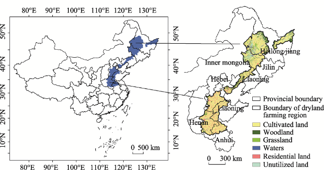
Figure 1 Distribution map of land use types in dryland farming region

2.2 Sampling

Study sites with a 15 km × 15 km grid distributed across the study region and dryland patches (including irrigated field) were extracted. The soil samples of DFR were taken from May to June in 2017. The sampling points are mainly placed on the black soil, black calcium soil, brown loam, tidal soil, brown soil, sandy ginger black soil and other six kinds of soil types with regard to the districts and counties, in relation to soil clay content level (0-5% for 1 level, 5% equal spacing, divided into 9 levels), planting system and other samplings, the sampling principle were comprehensively considered according to the size of the area and the degree of concentration. The details are that 1) each major soil type should have at least 20 sampling points, 2) each sub-category should as far as possible set up sampling points, 3) try to ensure that each clay grain level should have have sampling points distributed, and 4) try to ensure that each district and county should have one sampling point. The 0-40 cm soil layer is the part more frequently disturbed during tillage in DFR, it is also the part with higher organic carbon content and more obvious changes. Thus, in this study, the 0-40 cm depth was selected. Each sample was divided into four layers including 0-10 cm, 10-20 cm, 20-30 cm and 30-40 cm. A total of 1608 samples were collected from 402 locations of the DFR in 2017 (Figure 2). The soil samples were disposed by blending, natural air drying, grinding and sifting. The SOC, bulk density, pH and texture of soils were determined with potassium bichromate external heating, ring-knife, potential method and laser granulometry.
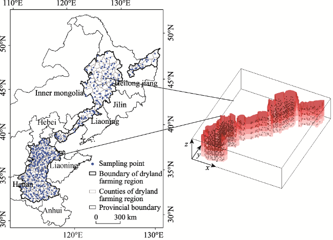
Figure 2 Spatial distribution of soil samples in dryland farming region

2.3 SOCD simulation

The calculation was conducted by the following equation.
$S O C D=\frac{S O C_{i} D_{i} E_{i}}{100}$
where SOCD is the soil organic carbon density at a certain depth (kg/m2); SOCi is the soil organic carbon content (g/kg); Di is the soil bulk density (g/cm3); Ei is the soil layer thickness with a value of certain depth.
Inverse distance weighting (IDW) was first proposed in the 1960s and is commonly applied to calculate regional precipitation (Zeng, 2013). IDW can accurately describe the three-dimensional spatial distribution characteristics of SOCD, while the Kriging method is unable to meet the assumption due to complex variations in the vertical direction of SOCD across the alluvial plain area (Chen et al., 2015). IDW relates the value of the interpolation point to distance, with smaller distances associated with greater impacts. The weight of the interpolated point value gradually decreases as the distance increases. This method has two main parameters, the number of search points and the vertical magnification. The search points are the number of known points near the selected unknown points. Since the study distance in the vertical direction (soil depth) was too small relative to the horizontal direction (sample spacing) for this study, the order of magnitude of the vertical direction was magnified in order to unify the order of magnitude of the sampling spacing in each direction, referred to as the vertical magnification multiple. IDW methods can be divided into two groups:
Shepard (SPD) was described in Eqs.2-4:
$V(x, y, z)=\sum_{i=1}^{n} w_{i} v_{i}\left(x_{i}, y_{i}, z_{i}\right)$
$w_{i}=\left(\frac{D-h_{i}}{D h_{i}}\right)^{2} / \sum_{i=1}^{n}\left(\frac{D-h_{i}}{D h_{i}}\right)^{2}$
$h_{i}=\sqrt{\left(x-x_{i}\right)^{2}+\left(y-y_{i}\right)^{2}+\left(z-z_{i}\right)^{2}}$
where V is the property value of the point to be evaluated; vi is the property value of the known observation point corresponding to coordinates (x, y, z) and (xi, yi, zi); wi is the weight coefficient corresponding to the known point; hi is the distance from the unknown point to the known point; D is the maximum value of the nth known point to the unknown point; hi is the distance from the interpolation position to the ith point; and n is the total number of interpolating points (Franke, 1982).
The gradient plane nodal function (GPNF) can be described as follows:
$F(x, y, z)=\sum_{i=1}^{n} W_{i} Q_{i}(x, y, z)$
where Wi is the weighting factor of the corresponding known point; Qi is a node function or a function at a measuring point (Franke, 1982; Watson and Philip, 1985; Franke and Nielson, 2010). The value at the interpolation location is calculated as a weighted average value of each node function at that location. The standard form of SPD method can be considered as a special case of GPNF method in which the node function employs a horizontal face (constant). The node function can be taken as a tilt plane through a data point, as described in Eq.6:
$Q_{i}(x, y, z)=f_{x}\left(x-x_{i}\right)+f_{y}\left(y-y_{i}\right)+f_{z}\left(z-z_{i}\right)+f_{i}$
where fx, fy, and fz are the partial derivatives of point estimated based on the geometry of surrounding points. The plane determined from Eq. 6 is denoted as a gradient plane. Each interpolation point is progressive at the point of measurement compared with the gradient plane, rather than close to the nearby original value. Furthermore, at least five non-common points must be used for the interpolation.

2.4 SOCS estimation

The three-dimensional simulation of the SOCD was performed using the GPNF method by GMS 10.4 (Aquaveo, Inc) at each point. The simulated results were imported into ArcGIS 10.3 (ESRI, Inc) and were superimposed on a distribution map to calculate the SOCS under different soil layer in each province of DFR.

2.5 SOCP estimation

The carbon sequestration potential of DFR was estimated for the 0-20 and 20-40 cm layers with the model, using the temperature, precipitation, soil clay content and pH as inputs. The annual average temperature and precipitation were taken as the average daily values from 2012 to 2016, while the annual average irrigation was based on the agricultural water quota standards of the provinces. The soil clay content and pH were measured in 2017. The model coefficients of line 164 were determined from 76 foreign long-term positioning experimental datasets. In order to model the carbon sequestration pallet of the soil, data from 95 long-term localization experiments on DFR were obtained from a global scale to form a database of long-term localization experiments. These experimental sites were located in temperate, subtropical and tropical climatic zones worldwide and had high inputs of exogenous organic carbon (stable manure or straw) (10-40 t/ha/year on average). Of these 95 long-term location trials, 22 lasted 10-14 years and 73 exceeded 15 years. The SOC measurement that reached saturation in the last years was assumed to be the SOCp value at that point, based on SOC variation (Qin and Huang, 2010).
$S O C_{P}=S S O C_{S}-S O C D$
$S S O C_{S}=140.5 \mathrm{e}^{-0.021 M T}-98.8 e^{-0.42 M P}-39.6 e^{-0.10 C L}-4.1 \mathrm{pH}-27.7$
where SOCP is the soil organic carbon sequestration potential of sample (kg/m2); SSOCS is saturated soil organic carbon density of sample (kg/m2); SOCD is the soil organic carbon density at a 20 cm depth of sample (kg/m2); MT and MP are the annual average temperature (℃) and total precipitation and irrigation (mm) respectively; CL is clay content (%); and pH represents soil pH.
According to the model, SOCP and SSOCS of each sampling point were calculated, and the Kriging interpolation method was used to map the spatial distribution of SOCS, SOCD, and SOCP in the study area, and the SOCP and SOCSS in DFR were calculated by raster.

3 Results

3.1 Optimization of the three-dimensional simulation

(1) Effect of search points on interpolation
The SOCD decreased with increased soil depth, while the interpolation smoothness increased with the number of search points (Figure 3). The characteristics of vertical gradient distribution were more prominent simulated by GPNF than the characteristics simulated by SPD. The SOCD change of vertical direction was inconspicuous simulated by traditional SPD method, meanwhile, interpolation results were smoother and less “bull’s eye”. There was a significant change of the interpolation results when n increased from 2 to 15, while few differences were observed when n values increased from 15 to 25. Compared with the results simulated by GPNF, interpolation results became vertically homogenized as the number of search points increased simulated by traditional SPD.
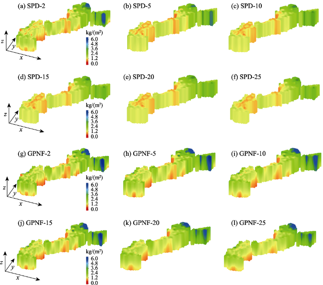
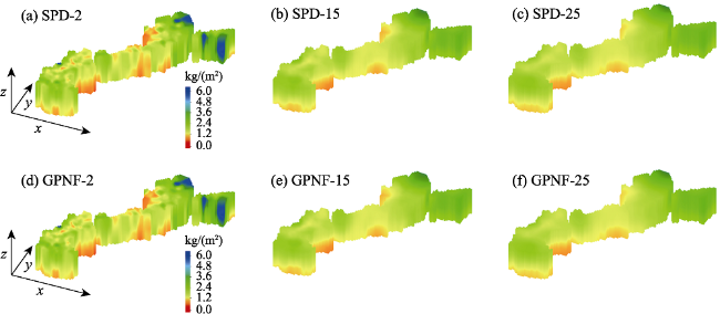
Figure 3 Spatial distribution of SOCD with different methods and search points

Note: the number after the method represents the number of search points.

The average square root error of SOCD fluctuated significantly with increasing n values from 0 to 5 under all layers, a smoother trend occurred for n values from 5 to 10 and a subsequent stable change appeared for n from 15 to 25. The minimum average square root error of the soil SOCD was observed at search point 25 under each layer. At the depth layer of 40 cm, the average square root error of SOCD was 0.51 and 0.55 for GPNF and SPD, respectively (Figure 4).
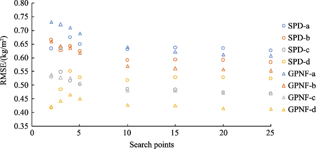
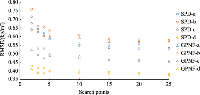
Figure 4 The relation between RMSE and search points under different methods

Note: a, b, c and d represent the 0-10 cm, 10-20 cm, 20-30 cm and 30-40 cm soil layers, the same below.

(2) Effect of vertical magnification on interpolation
The interpolation results are generally in agreement with the pre-amplification at the vertical magnification multiple of 1.0×10⁶ and search point of 2, respectively. However, the interpolation results became smoother with increasing search points and disappearing “bull’s-eye” simulated by GPNF model, while vertical differentiation characteristics were observed by traditional SPD method (Figure 5). Thus, increasing the vertical magnification can improve the interpolation effect simulated by traditional SPD method.
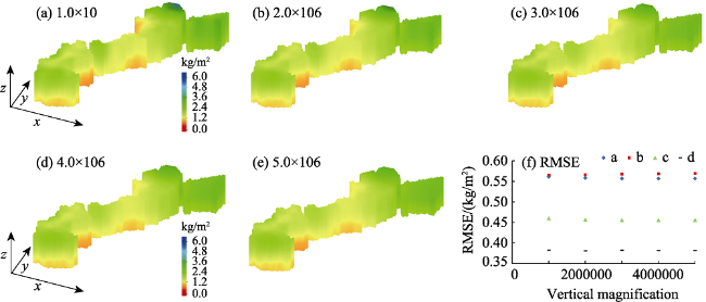
Figure 5 Spatial distribution of SOCD with different methods and search points under a magnification of 1.0×10⁶
As the search points increased, the average square root error of SOCD significantly fluctuated (n equal to 0-5), followed by a smoother trend (n equal to 5-10) until values became stable (n equal to 15-25) across all layers. The minimum average square root error of SOCD was observed at the search point of 25 for each layer, while the average soil square root errors at the 0-40 cm layer were determined as 0.48 and 0.49 for the GPNF and traditional SPD methods, respectively. Thus, the GPNF method was used to further investigate the effect of vertical magnification on the SOCD interpolation results for the number of search points equal to 25 (Figure 6).
Figure 6 Relation between RMSE and search points under SPD and GPNF with a magnification of 1.0×10⁶
When the number of search points was 25 and the interpolation method was GPNF method, the 3D simulation effect of SOCD was consistent across magnifications under each layer. The mean square root error decreased with the soil layer depth, while few differences were observed across magnifications (Figure 7). There was no significant difference among the root mean square error under different vertical magnification for each layer in DFR.
Figure 7 Spatial distribution and RMSE of SOCD by GPNF method with different vertical magnifications

3.2 Uncertainty analysis

Figure 8 presents the uncertainty of the SPD and GPNF methods across different magnification values. Under the 0-10 cm and 10-20 cm soil layers, the simulated variance exhibited a decreasing trend as the magnification increased from 1.0×10⁶ to 3.0×10⁶. In contrast, the simulated variance was constant for magnification values from 3.0×10⁶ to 6.0×10⁶ as the soil depth increased. The GPNF-simulated SOCD variances were 0.21, 0.28, 0.36 and 0.32, while the equivalent SPD values were determined as 0.21, 0.30, 0.38 and 0.33 under each layer, respectively. Total variances of 0.29 and 0.31 were calculated by GPNF and SPD, respectively. The SOCD 3D spatial simulation uncertainties determine the GPNF to be more accurate than the SPD method for the number of search points equal to 25 and a magnification of 3.0×10⁶.
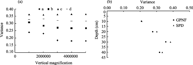
Figure 8 Variance of SPD and GPNF methods with different magnification values

3.3 Spatial distribution of SOCD, SSOCS and SOCP under different soil layers

SOCD, SSOCS and SOCP in the Northeast China DFR exceeded those in the Huang-Huai-Hai DFR (Figures 9a-9c). The magnitude of SOCS and SSOCS decreased with increasing soil depth across DFR (Figures 9d and 9e). Despite high SOCD in Northeast China, the positive values of the SOCP in the region indicate the fixing of carbon as a carbon sink, principally in the southern part of Heilongjiang province, across most of Jilin province and the north-central Liaoning province. The carbon sink areas exhibited an increasing trend with depth for the 20-40 cm soil layer, as well as central Heilongjiang. However, the rest of Northeast China was revealed as a carbon sink, some areas of the Huang-Huai-Hai also change from carbon sources to carbon sinks (Figure 9f).
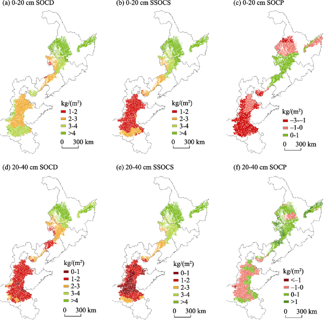
Figure 9 Spatial distribution characteristics of SOCD, SSOCS and SOCP in dryland farming region

Note: SOCD, SSOCS and SOCP represent the SOCS, SSOCS and SOCP of each sampling site, respectively.

3.4 SOCS under different soil layers

The existing SOCS under the 0-20 cm and 20-40 cm soil layers for DFR were estimated as 13.12×10¹¹ kg and 9.16×10¹¹ kg. The three-dimensional interpolation of SOCS with the values of 6.63×10¹¹ kg, 6.49×10¹¹ kg, 5.01×10¹¹ kg, and 4.15×10¹¹ kg for soil layers from 0-10 cm to 0-40 cm, respectively (Table 1). The highest SOCS was associated with Heilongjiang province, with the value ranging from 2.26×10¹¹ kg to 3.18×10¹¹ kg under different soil layers, followed by Henan and Jilin provinces, while the lowest SOCS was estimated in Liaoning and Shandong provinces. The SOCS decreased with increasing soil depth for all provinces, except Heilongjiang and Jilin provinces, the principal distribution areas of black soil in China.
Table 1 SOCS estimated by GPNF under different soil levels in dryland farming region of each province
Province SOCS
0-10 cm 10-20 cm 20-30 cm 30-40 cm 0-40 cm 0-20 cm 20-40 cm
(1011 kg) (1011 kg) (1011 kg) (1011 kg) (1011 kg) (1011 kg) (1011 kg)
Jilin 0.69 0.83 0.65 0.60 2.77 1.52 1.25
Liaoning 0.32 0.29 0.26 0.20 1.07 0.61 0.46
Anhui 0.58 0.35 0.31 0.19 1.43 0.93 0.49
Shandong 0.54 0.39 0.27 0.18 1.38 0.93 0.45
Heilongjiang 2.51 3.18 2.35 2.26 10.30 5.69 4.61
Hebei 0.87 0.63 0.51 0.34 2.35 1.5 0.85
Henan 1.12 0.82 0.66 0.38 2.98 1.94 1.04
Total 6.63 6.49 5.01 4.15 22.28 13.12 9.16

3.5 SOCS, SSOCS and SOCP under different soil layers and provinces

The SOCP of DFR exhibited negative, except Jilin and Liaoning provinces (Table 2). Henan Province played the most obvious “carbon source” role, followed by Hebei, Heilongjiang, Shandong, and Anhui provinces (Table 2). The existing SOCS was determined as 9.16×10¹¹ kg under 20-40 cm soil layer in DFR, while saturated soil organic carbon storage (SSOCS) and SOCP were estimated as 10.17×10¹¹ kg and 0.95×10¹¹ kg, respectively, indicating an overall carbon sink performance. SOCP was positive across DFR, except Shandong, Henan and Hebei. Heilongjiang was determined as the most significant carbon sink, followed by Jilin, Liaoning and Anhui.
Table 2 SOCS, SSOCS and SOCP estimated by GPNF under different soil levels in each province of DFR
Province SOCS SSOCS SOCP
0-20 cm 20-40 cm 0-20 cm 20-40 cm 0-20 cm 20-40 cm
(1011 kg) (1011 kg) (1011 kg) (1011 kg) (1011 kg) (1011 kg)
Jilin 1.52 1.25 1.71 1.67 0.19 0.44
Liaoning 0.61 0.46 0.72 0.70 0.11 0.21
Anhui 0.93 0.49 0.57 0.50 -0.36 0.02
Shandong 0.93 0.45 0.54 0.43 -0.39 -0.01
Heilongjiang 5.69 4.61 5.26 5.24 -0.43 0.56
Hebei 1.50 0.85 0.89 0.79 -0.61 -0.05
Henan 1.94 1.04 0.94 0.82 -1.00 -0.21
Total 13.12 9.16 10.63 10.17 -2.49 0.95

4 Discussion

Compared to the traditional SPD method, the GPNF method is able to better simulate the vertical distribution characteristics of SOCD without increasing the vertical magnification. This is attributed to the inclusion of the gradient distribution characteristics of the original data for the GPNF interpolation, whereas the traditional SPD method simply takes distance as the weight. Therefore, the homogenization observed in the vertical direction indicated the greater ability of the GPNF method to simulate the spatial characteristics with the gradient trend distribution.
Increasing the vertical magnification was able to better demonstrate the interpolation. This study employed a 40-cm soil layer thickness and a 20 to 50 km sampling point spacing in the horizontal direction, while the vertical distance was only 10 cm, and the vertical direction of the sampling spacing is only horizontal direction of 5×10⁻⁶ to 2×10⁻⁶. The denominator of Eq. 3 is invariant when the number of search points is known, splitting the molecular component into the following expression:
$\left(\frac{D-h_{i}}{D h_{i}}\right)^{2}=\frac{D^{2}-2 D h_{i}+h_{i}^{2}}{D^{2} h_{i}^{2}}=\frac{1}{h_{i}^{2}}-\frac{2}{D h_{i}}+\frac{1}{D^{2}}$
where the smaller the spacing between the sampling points in the horizontal direction, the smaller the value hi and the larger the weight coefficient corresponding to the measured points. For the points to be interpolated, the weight of vertical points in item 1 is 4×10¹⁰-2.5×10¹¹ times the weight of neighboring points in the horizontal direction, and the weight of vertical points in item 2 is 2.0×10⁵-5.0×10⁵ times the weight of neighboring points in the horizontal direction, thus it can be seen that the overall weight is mainly in item 1, which leads to no difference of interpolation result in the vertical direction. Therefore, the traditional SPD method is unable to perform the three-dimensional inverse distance-weighted interpolation of the soil profile SOCD without increasing the vertical magnification. This is in agreement with previous literature (Chen et al., 2015).
By taking into account the vertical distribution characteristics of the study data, the GPNF method with vertical magnification eliminates the effects of large differences in the vertical to horizontal distance ratio on the spatial interpolation, increasing the accuracy of the simulation. Here, we provide a preliminary discussion of the results. Further research is required to determine whether the method is suitable for additional soil properties and to evaluate its application across different scales.
Heilongjiang, Jilin and Liaoning provinces proved to be rich regions in terms of SOCS, with values in Heilongjiang and Jilin decreasing less with an increasing soil depth. This is linked to the key roles played by the two provinces in the distribution of black soil in China. In particular, the colder climate prevents the rapid decomposition of soil organic matter, resulting in thicker black soil tillage layers and higher soil organic matter content, which is consistent with previous work (Xie et al., 2004; Ren et al., 2013).
One of the main reasons for the difference in carbon sequestration potential between the Northeast DFR and the Huang-Huai-Hai DFR is that the recent organic carbon content in the Northeast black soil area has decreased significantly, while the recent organic carbon content in the Huang-Huai-Hai DFR has shown an increasing trend, so the carbon sequestration potential in the Northeast DFR is higher than that in the Huang-Huai-Hai DFR. The carbon saturation model determined the SOCP at 0-20 cm soil layer to be positive for a DFR of Jilin and part of Liaoning. This is consistent with previous research (Yang, 2016), indicating that under the current environmental conditions, the region will become a carbon sink, and should thus strengthen farmland management by supporting relevant fertilizer technology, farmer training, government subsidies, as well as returning straw to the field and other measures to improve the soil organic carbon content (Ma et al., 2021).
Negative SOCP values were determined for several areas of the Huang-Huai-Hai Plain and Heilongjiang province, contradicting previous work (Guo, 2015; Liu, 2011). This is attributed to the following reasons: 1) The artificial management of fertilizer measures employed to increase the region's soil organic carbon content has risen in recent years, while SOCD data from previous studies is based on the years 1980-2000. 2) The irrigation amount used in the model was set as the irrigation quota of the provinces, while the farmers irrigated more, resulting in an underestimation of the SOCP. 3) In the long-term localization experimental data used for the modeling, the carbon input at some experimental sites did not reach the theoretical maximum, reducing the soil carbon saturation level (Qin and Huang, 2010). In the 20 to 40 cm soil layer, the SOCP of DFR was determined as a carbon sink, indicating the carbon sequestration potential of the soil in this layer. In order to take full advantage of the carbon sequestration effect, the organic carbon content in this layer should be improved.
In this paper, we only compared the simulation accuracy between the isotropic GPNF method and the traditional SPD method on the basis of SOCD on a large scale. Research on aspects, such as the accuracy of simulations at different scales and on different soil properties, need to be further explored. The carbon sequestration potential of surface soils in DFR is only a preliminary estimation, however, the selection of parameters and weights of this carbon saturation model in different soil layers of different regions still need further study.

5 Conclusions

(1) The SOCD spatial distribution characteristics were more accurately simulated by GPNF method compared to the traditional SPD method without magnifying the vertical multiples. Increasing the vertical magnification can successfully improve the interpolation effect of the traditional SPD method. The GPNF optimizes the simulated effect of SOCD for vertical magnification multiples greater than 3.0×10⁶ and a number of search points equal to 25 under each layer in DFR.
(2) At 0-40 cm and 0-20 cm soil layers, the GPNF-derived SOCS were estimated as 22.28×10¹¹ kg and 13.12×10¹¹ kg, respectively, in DFR.
(3) The proposed model for farmland soil carbon sequestration determined the SOCP as 0.95×10¹¹ kg at 20-40 cm soil layer in DFR. This indicates the region to be a carbon sink, with the exception of DFR in Shandong, Henan and Hebei provinces. Future SOCP values were predicted to be positive, of which the carbon sink effect is most obvious in Heilongjiang province. In particular, SOCP values in DFR were estimated as -2.49×10¹¹ kg for the 0 to 20 cm soil layer and were thus considered as a carbon source. Jilin and Liaoning provinces were identified as carbon sinks based on their predicted SOCP values, while the remaining provinces were considered as carbon sources.
(4) These observations are preliminary estimates of the carbon sequestration potential at the surface soil across the study area. The results demonstrated the shift of the 0-20 cm soil layer in DFR from a carbon sink to a carbon source. Thus, the SOCD content of the area should be closely monitored.
[1]
Alidoust E, Afyuni M, Hajabbasi M A et al., 2018. Soil carbon sequestration potential as affected by soil physical and climatic factors under different land uses in a semiarid region. Catena, 171: 62-71.

DOI

[2]
Angers D A, Arrouays D, Saby N P A et al., 2011. Estimating and mapping the carbon saturation deficit of French agricultural topsoils. Soil Use and Management, 27(4): 448-452.

DOI

[3]
Bayer C, Lovato T, Dieckow J et al., 2006. A method for estimating coefficients of soil organic matter dynamics based on long-term experiments. Soil and Tillage Research, 91(1/2): 217-226.

DOI

[4]
Berg E V D, Reich P, 1993. Organic carbon in soils of the world. Soil Science Society of America Journal, 57(4): 269-273.

[5]
Castrignanò A, Maiorana M, Fornaro F et al., 2002. 3D spatial variability of soil strength and its change over time in a durum wheat field in southern Italy. Soil & Tillage Research, 65(1): 95-108.

[6]
Chen C, Hu K, Li H et al., 2015. Three-dimensional mapping of soil organic carbon by combining kriging method with profile depth function. Plos One, 10(6): e129038.

[7]
Chung H, Grove J H, Six J, 2008. Indications for soil carbon saturation in a temperate agroecosystem. Soil Science Society of America Journal, 72(4): 1132-1139.

DOI

[8]
Du Z, Wu W, Zhang Q et al., 2014. Long-term manure amendments enhance soil aggregation and carbon saturation of stable pools in North China Plain. Journal of Integrative Agriculture, 13(10): 2276-2285.

DOI

[9]
Fang J, Yu G, Ren X et al., 2015. Carbon sequestration in China's terrestrial ecosystems under climate change: Progress on ecosystem carbon sequestration from the cas strategic priority research program. Bulletin of Chinese Academy of Sciences, 30(6): 848-857. (in Chinese)

[10]
Franke R, 1982. Scattered data interpolation: Tests of some method. Mathematics of Computation, 38(157): 181-200.

[11]
Franke R, Nielson G, 2010. Smooth interpolation of large sets of scatter data. International Journal for Numerical Methods in Engineering, 15(11): 1691-1704.

DOI

[12]
Grant R F, Juma N G, Robertson J A et al., 2001. Long-term changes in soil carbon under different fertilizer, manure, and rotation. Soil Science Society of America Journal, 65(1): 205-214.

DOI

[13]
Guo J, 2015. Study on soil carbon reservoir change and carbon sequestration potential in typical areas of the Yangtze River Basin[D]. Beijing: China University of Geosciences. (in Chinese)

[14]
Kamoni P T, Gicheru P T, Wokabi S M et al., 2007. Evaluation of two soil carbon models using two Kenyan long term experimental datasets. Agriculture, Ecosystems & Environment, 122(1): 95-104.

DOI

[15]
Kumar S, Lal R, Liu D et al., 2013. Estimating the spatial distribution of organic carbon density for the soils of Ohio. Journal of Geographical Sciences, 23(2): 280-296.

DOI

[16]
Lacoste M, Minasny B, Mcbratney A et al., 2014. High resolution 3D mapping of soil organic carbon in a heterogeneous agricultural landscape. Geoderma, 213(1): 296-311.

DOI

[17]
Lal R, 2004. Soil carbon sequestration impacts on global climate change and food security. Science, 304(5677): 1623-1627.

PMID

[18]
Liu F, Zhang G, Sun Y et al., 2013. Mapping the three-dimensional distribution of soil organic matter across a subtropical hilly landscape. Soil Science Society of America Journal, 77(4): 1241.

DOI

[19]
Liu H, 2011. Dynamic change of soil organic carbon and estimation of carbon sequestration potential in Liaoning province[D]. Shenyang: Shenyang Agricultural University. (in Chinese)

[20]
Ma W, Zhan Y, Chen S et al., 2021. Organic carbon storage potential of cropland topsoils in East China: Indispensable roles of cropping systems and soil managements. Soil and Tillage Research, 211(Suppl. 1): 105052.

[21]
Malone B P, Mcbratney A B, Minasny B et al., 2009. Mapping continuous depth functions of soil carbon storage and available water capacity. Geoderma, 154(1): 138-152.

DOI

[22]
Minasny B, Mcbratney A B, Mendonça-Santos M L et al., 2006. Prediction and digital mapping of soil carbon storage in the Lower Namoi Valley. Soil Research, 44(3): 233-244.

DOI

[23]
Mishra U, Lal R, Slater B et al., 2009. Predicting soil organic carbon stock using profile depth distribution functions and ordinary kriging. Soil Science Society of America Journal, 73(2): 614-621.

DOI

[24]
Pan G, Lu H, Li L et al., 2015. Soil carbon sequestration with bioactivity: A new emerging frontier for sustainable soil management. Advances in Earth Science, 30(8): 940-951.

[25]
Qin Z, Huang Y, 2010. Quantification of soil organic carbon sequestration potential in cropland: A model approach. Science China Life Sciences, (7): 658-676.

[26]
Ren C, Zhang C, Wang Z et al., 2013. Organic carbon storage and sequestration potential in cropland surface soils of Songnen Plain maize belt. Journal of Natural Resources, 28(4): 596-607. (in Chinese)

[27]
Schmidt M W, Torn M S, 2011. Persistence of soil organic matter as an ecosystem property. Nature, 478(7367): 49-56.

DOI

[28]
Singh N R, Kumar D, Rao K K et al., 2020. Agroforestry:Soil organic carbon and its carbon sequestration potential.In: Climate Change and Agroforestry Systems. Boca Raton: Apple Academic Press. https://doi.org/10.1201/9780429286759-5.

[29]
Singh S K, Singh A K, Sharma B K et al., 2007. Carbon stock and organic carbon dynamics in soils of Rajasthan, India. Journal of Arid Environments, 68(3): 408-421.

DOI

[30]
Six J, Conant R T, Paul E A et al., 2002. Stabilization mechanisms of soil organic matter: Implications for C-saturation of soils. Plant and Soil, 241(2): 155-176.

DOI

[31]
Stewart C E, Paustian K, Conant R T et al., 2008. Soil carbon saturation: Evaluation and corroboration by long-term incubations. Soil Biology and Biochemistry, 40(7): 1741-1750.

DOI

[32]
Sun Z, Li Y, Zhao Y et al., 2019. Analysis on spatial distribution characteristics and driving forces of soil organic carbon density in dry farming region. Transactions of the Chinese Society for Agricultural Machinery, 50(1): 255-262. (in Chinese)

[33]
Van Meirvenne M, Maes K, Hofman G, 2003. Three-dimensional variability of soil nitrate-nitrogen in an agricultural field. Biology and Fertility of Soils, 37(3): 147-153.

DOI

[34]
Veronesi F, Corstanje R, Mayr T, 2012. Mapping soil compaction in 3D with depth functions. Soil & Tillage Research, 124(4): 111-118.

[35]
Wang Y, Liu K, Wu Z et al., 2020. Comparison and analysis of three estimation methods for soil carbon sequestration potential in the Ebinur Lake Wetland, China. Frontiers of Earth Science, 14(1): 13-24.

DOI

[36]
Waqas M A, Li Y, Smith P et al., 2020. The influence of nutrient management on soil organic carbon storage, crop production, and yield stability varies under different climates. Journal of Cleaner Production, 268: 121922.

DOI

[37]
Watson D F, Philip G M, 1985. A refinement of inverse distance weighted interpolation. Geoprocessing, 2(2): 315-327.

[38]
West T O, Marland G, King A W et al., 2004. Carbon management response curves: Estimates of temporal soil carbon dynamics. Environmental Management, 33(4): 507-518.

[39]
Xie R, X Wu, 2016. Effects of grazing intensity on soil organic carbon of rangelands in Xilin Gol League, Inner Mongolia, China. Journal of Geographical Sciences, 26(11): 1550-1560.

DOI

[40]
Xu L, Yu G, He N, 2019. Increased soil organic carbon storage in Chinese terrestrial ecosystems from the 1980s to the 2010s. Journal of Geographical Sciences, 29(1): 49-66.

DOI

[41]
Yang K, 2016. Carbon sequestration potential of soil in typical agricultural areas in China[D]. Beijing: China University of Geosciences. (in Chinese)

[42]
Yang S, Malhi S S, Li F et al., 2007. Long-term effects of manure and fertilization on soil organic matter and quality parameters of a calcareous soil in NW China. Journal of Plant Nutrition and Soil Science, 170(2): 234-243.

DOI

[43]
Yao J, Kong X, 2018. Modeling the effects of land-use optimization on the soil organic carbon sequestration potential. Journal of Geographical Sciences, 28(11): 1641-1658.

DOI

[44]
Young R R, Wilson B, Harden S et al., 2009. Accumulation of soil carbon under zero tillage cropping and perennial vegetation on the Liverpool Plains, eastern Australia. Soil Research, 47(3): 273.

DOI

[45]
Zeng F, 2013. Study on statistical inference method of three dimensional interpore geological characteristics[D]. Guangzhou: South China University of Technology. (in Chinese)

[46]
Zheng J, Cheng K, Pan G et al., 2011. Perspectives on studies on soil carbon stocks and the carbon sequestration potential of China. Chinese Science Bulletin, (26): 2162-2173. (in Chinese)

[47]
Zhu W, Zhang J, Cui Y et al., 2020. Ecosystem carbon storage under different scenarios of land use change in Qihe catchment, China. Journal of Geographical Sciences, 30(9): 1507-1522.

DOI

Outlines

/