Special Issue: Ecohydrology

Quantification of human and climate contributions to multi-dimensional hydrological alterations: A case study in the Upper Minjiang River, China

  • ZHANG Yuhang , 1 ,
  • YE Aizhong , 1, * ,
  • YOU Jinjun 2 ,
  • JING Xiangyang 3
Expand
  • 1. State Key Laboratory of Earth Surface Processes and Resource Ecology, Institute of Land Surface System and Sustainable Development, Faculty of Geographical Science, Beijing Normal University, Beijing 100875, China
  • 2. State Key Laboratory of Simulation and Regulation of Water Cycle in River Basin, China Institute of Water Resources and Hydropower Research, Beijing 100038, China
  • 3. POWERCHINA Chengdu Engineering Corporation Limited, Chengdu 611130, China
*Ye Aizhong (1978-), Professor, specialized in hydrological model. E-mail:

Zhang Yuhang (1994-), specialized in hydrometeorological ensemble forecast. E-mail:

Received date: 2020-08-26

  Accepted date: 2021-03-09

  Online published: 2021-10-25

Supported by

Natural Science Foundation of China(51879009)

Natural Science Foundation of China(52079143)

Second Tibetan Plateau Scientific Expedition and Research Program(2019QZKK0405)

National Key Research and Development Program of China(2018YFE0196000)

National Key Research and Development Program of China(2017YFC0404405)

Interdisciplinary Research Foundation of Beijing Normal University for the First-Year Doctoral Students(BNUXKJC1905)

Independent Research Projects of POWERCHINA Chengdu Engineering Corporation Limited(P34516)

Abstract

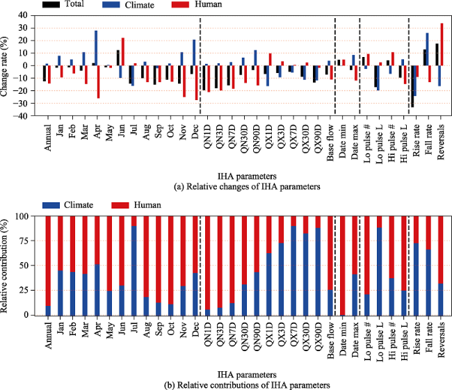
Dual factors of climate and human on the hydrological process are reflected not only in changes in the spatiotemporal distribution of water resource amounts but also in the various characteristics of river flow regimes. Isolating and quantifying their contributions to these hydrological alterations helps us to comprehensively understand the response mechanism and patterns of hydrological process to the two kinds of factors. Here we develop a general framework using hydrological model and 33 indicators to describe hydrological process and quantify the impact from climate and human. And we select the Upper Minjiang River (UMR) as a case to explore its feasibility. The results indicate that our approach successfully recognizes the characteristics of river flow regimes in different scenarios and quantitatively separates the climate and human contributions to multi-dimensional hydrological alterations. Among these indicators, 26 of 33 indicators decrease over the past half-century (1961-2012) in the UMR, with change rates ranging from 1.3% to 33.2%, and the human impacts are the dominant factor affecting hydrological processes, with an average relative contribution rate of 58.6%. Climate change causes an increase in most indicators, with an average relative contribution rate of 41.4%. Specifically, changes in precipitation and reservoir operation may play a considerable role in inducing these alterations. The findings in this study help us better understand the response mechanism of hydrological process under changing environment and is conducive to climate change adaptation, water resource planning and ecological construction.

Cite this article

ZHANG Yuhang , YE Aizhong , YOU Jinjun , JING Xiangyang . Quantification of human and climate contributions to multi-dimensional hydrological alterations: A case study in the Upper Minjiang River, China[J]. Journal of Geographical Sciences, 2021 , 31(8) : 1102 -1122 . DOI: 10.1007/s11442-021-1887-z

1 Introduction

In recent years, with the increase in carbon emissions, climate warming has been observed, and even a more extreme warming condition is projected for the future by climate models at both global and regional scales (Zhou et al., 2014; Sun et al., 2015; Donat et al., 2016; Wu et al., 2016). On the other hand, with increasing water demands, human activities have significantly altered the natural river flow condition in various ways, such as dam and reservoir construction (Li et al., 2010; Yang et al., 2011), water withdrawal (Liu et al., 2014), land-use change (Shrestha and Htut, 2016) and groundwater pumping. As a key link among the atmosphere, hydrosphere and biosphere, there is ample evidence that the hydrological process is being affected by dual factors from climate and human. For example, more extreme rainfall events can cause more extreme floods (De Luca et al., 2019). The spatiotemporal patterns of river discharge may be affected by dam construction and reservoir operation (Talukdar and Pal, 2019). All these changes are reflected not only in changes in total water storage (Liu et al., 2012) but also in multiple dimensions of river flow regimes (Mittal et al., 2016). Moreover, these changes may cause huge effects on river ecosystems (Kundzewicz, 2008). Therefore, systematic assessment of hydrological alterations must adopt multiple indicators instead of one single indicator at the watershed scale. So as to better serve decision-makers to develop better strategies and policies for climate change adaptation, ecosystem protection and integrated watershed management.
In general, there are two factors (climate and human) that cause the change of land surface hydrological process. Many case studies and methodological discussions have been carried out by researchers at various watersheds and time scales (Ma et al., 2010; Ma et al., 2014; Xin et al., 2019). Three kinds of methods are widely used, namely, empirical models, climate elastic models, and hydrological modelling-based approaches. The empirical method is used to establish the statistical relationship between climate variables and runoff, and to quantify the natural and human contributions by comparing the differences of this relationship in different periods, and analyses of these models include linear regression model, time-variant analyses, and the double cumulative curve. For example, Zhao et al. (2014) attributed the annual streamflow changes using the linear regression model, and the results indicated that climate change, especially the decrease in rainfall, caused a decrease in runoff. Climate elastic models are mainly based on the various solutions of the Budyko hypothesis (Wu et al., 2016). The hydrological modelling-based approaches abstract complicated physical mechanisms into mathematical equations to simulate the land surface hydrological process. By simulating the runoff process under different meteorological or underlying surface conditions, the relative contribution of climate change and human impacts can be estimated. For example, a geomorphology-based hydrological model (GBHM) was used in the Miyun Reservoir, and the results revealed that the factor of climate and human accounted for 55% and 18% for the decrease in reservoir discharge, respectively (Ma et al., 2010). Some researchers also compared these different methods. Theoretical analysis including methodologies, assumptions and preconditions, and a series of calculations and applications by using different methods were discussed and conducted (Wang, 2014; Dey and Mishra, 2017; Wu et al., 2017). The common conclusion from all these studies is that although the hydrological model has some structural errors and needs to be further improved, the method by using the hydrological model has more advantages than other methods because of its physical mechanism. What's more, it can also be used in the context of a changing environment. And the hydrological modelling-based approach is required as such an approach can generate time-series data for multiple hydrological variables. Therefore, it is considered to be the most promising approach among the various methods. In this study, the hydrological model is used to simulate the natural river flow condition during the altered period at the daily scale and can therefore satisfy our demand to assess the hydrological alterations at multiple dimensions. However, most previous studies mainly focused on total water storage or discharge at annual or seasonal scales (Jiang et al., 2017). Changes in natural flow regime characteristics have not been fully investigated.
Among the metrics for describing the various characteristics of flow regimes, the indicators of hydrological alterations (IHA) method has been commonly used and further developed to assess hydrological alterations in the context of watersheds that are disrupted by different anthropogenic influences and climate change scenarios (Yang et al., 2017). Wang et al. (2017) took four different watersheds as a case study and addressed the IHA method to comprehensively analyze hydrological alterations using Coupled Model Intercomparison Project Phase 5 (CMIP5) climate scenarios. On the other hand, the hydrological impacts caused by large dam construction were also studied and quantified by the IHA method (Yang et al., 2008; Zhao et al., 2012). In addition, the small hydropower-developed region such as Jiulong River basin was examined, and cumulative effects of intense small dam construction were quantified by the IHA method (Lu et al., 2018). However, these studies only concentrated on quantitatively assessing changes in the river flow regimes under one single factor of climate or human. There are relatively few studies on the simultaneous quantification of the dual impacts and their contributions.
To solve the issues mentioned above, here we propose a framework using hydrological model and 33 indicators to describe hydrological alterations and quantify the impact from climate and human. As an important tributary of the Yangtze River, Minjiang River also experienced dual impacts from climate and human. In particular, the obvious stage of human activities development occurred in the Upper Minjiang River (UMR) (Hou et al., 2018), which meets our research needs. Therefore, we take the UMR as an example and use a distributed time-variant gain (DTVGM) hydrological model to explain the feasibility of our proposed framework and explore the ongoing hydrological alterations at the watershed scale. The information of the UMR and data are introduced in section 2. The proposed research framework, quantitative method, DTVGM hydrological model, and IHA parameters are provided in section 3. The results regarding the dual effects and the changes of IHA parameters are presented in section 4. An attribution analysis and possible ecological impacts of hydrological alteration are discussed in section 5. The conclusions follow at the end of this article.

2 Study area and data

2.1 Study area

As a part of the Chengdu Plain, the Minjiang River is located between the Sichuan Basin and the Qinghai-Tibet Plateau, China. And it is one of the primary tributaries of the Yangtze River. Here we select the Upper Minjiang River as a study area (Figure 1). The Upper Minjiang River (UMR) refers to the area between the headwaters of the Minjiang River and Dujiangyan Irrigation System and stretches from 102°45°E-103°96°E to 30°80°N-33°20°N. The UMR spans 341 km, with a total area of approximately 22,722 km2 and significant variation in elevation from north to south (from 5578 m to 726 m).
The UMR, the major water supply source, is an important ecological barrier in the Chengdu Plain. Affected by the subtropical monsoon, the mean annual precipitation (MAP) in the UMR is 987 mm with significant seasonality. The average, maximum, and minimum daily temperature are 11.3℃, 40℃, and 0℃, respectively. And the mean annual evaporation is 300 mm. As the control station of the UMR, the Zipingpu (ZPP) hydrological station has an annual average streamflow of 457 m3/s. Water for human activities includes agricultural irrigation and domestic and industrial production in the Chengdu Plain. The construction of hydroelectric power plants has altered the streamflow significantly (Zhang et al., 2012; Hou et al., 2018).
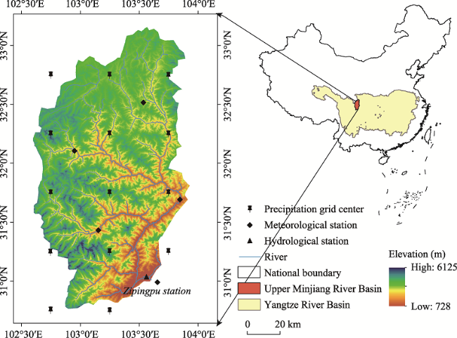
Figure 1 Location and attributes of the Upper Minjiang River

2.2 Data

The data mainly includes the following three categories for this research. The data sources and acquisition are summarized in the section of Data availability after the main text.
1) Meteorological forcing. A gridded daily precipitation data (spatial resolution: 0.5°×0.5°) generated from 2472 rain gauges, which has been commonly applied for various studies in recent years (Wu et al., 2016; Lu et al., 2017). Wind speed, maximum and minimum temperature were collected from six national weather stations in the UMR or nearby areas (Figure 1). The time period of these data is from 1961 to 2012. For hydrological modelling, the precipitation and temperature data were further interpolated into each sub-basin by using the inverse distance weighting (IDW) method (Xu et al., 2018). The wind speed data was also interpolated into each sub-basin using the synergistic mapping (SYMAP) algorithm (Shepard, 1984).
2) Streamflow data. Daily (1961-2012) and monthly (1938-2012) streamflow records for the ZPP hydrological station were collected and used for long-term mutation diagnosis and model verification.
3) Watershed attribute information. Digital elevation model (DEM) data (~90 m), land use (~1 km) and soil type (~1 km) were collected and used to describe the spatial variability of the underlying surface of the watershed.

3 Methodologies

Our framework is briefly illustrated in Figure 2. First, observed streamflow data were collected and mutation diagnosis was carried out to segregate the study period into two periods (baseline and altered). Second, the DTVGM was set up, calibrated and verified in the first period, and natural streamflow during the altered period was reconstructed. Then, the change rate of IHA parameters and the climate and human contributions were calculated by comparing the observation and simulation during the baseline and altered periods. Finally, attribution analysis and the possible ecological impacts of hydrological alterations were discussed.
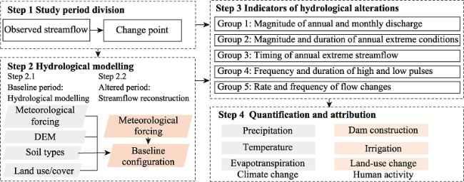
Figure 2 Framework of this study

3.1 Mutation diagnosis and study period division

To conduct our study, the first task is to detect the “change point” and define a “reference” period and a “change” period. Because the changes caused by human relatively larger than climate, the “change point” is often attributed to intense human activities, such as dam construction. During the baseline period, we assume that the hydrological alterations are mainly aroused by climate change while neglecting the human impacts. During the altered period, the hydrological alterations can be attributed to the dual effects of human and climate. There are two widely used methods to identify a “change point”. The first one is “human- designed”, in which the “change point” is identified artificially by data investigation and field investigation. The second one is to use a statistical test to distinguish hydrological variation, including the Mann-Kendall test (M-K test), the Pettitt test, and the double-mass curve test.
The M-K test (Mann, 1945; Kendall, 1948) is a nonparametric test method, which is easy to operate and widely used. Therefore we use this approach to catch the “change point” and verify its rationality through data investigation.
Given a hydrological streamflow record X with n samples, we are going to denote the X = x1, x2,, xn; And then, the rank statistic S of the M-K test can be conducted by Equations (1)-(3). And the expectation and variance of S can be calculated by Equations (4) and (5).
${{S}_{j}}=0,\ (j=1)$
${{S}_{j}}=\underset{k=1}{\overset{j}{\mathop \sum }}\,{{r}_{i}},(j=2,3,\ldots,n)$
${{r}_{i}}=\left\{ \begin{align} & 1,\ {{x}_{i}}>{{x}_{j}} \\ & 0,\ {{x}_{i}}<{{x}_{j}} \\ \end{align} \right.$
$E({{s}_{j}})=\frac{n(n+1)}{4}$
$Var({{s}_{j}})=\frac{n(n-1)(2n+5)}{72}$
Assuming that the time series is random and independent, we further define the statistics UFj by Equations (6) and (7).
$U{{F}_{j}}=0,(j=1)~$
$U{{F}_{j}}=\frac{{{S}_{j}}-E({{S}_{j}})}{\sqrt{Var({{S}_{j}})}},(j=2,3,\cdots,n)$
At a specified significance level α, if |UFj| is greater than Ua, the original hypothesis is accepted, and when UFj is greater (or smaller) than 0, there exists an increasing (or decreasing) trend. On the contrary, if |UFj| is less than Ua, the original hypothesis is rejected, that is no trend existing in sequences.
Similarly, we calculate the statistics UBj using the reversed X. We plot UF and UB curves in the same coordinate system. If there is an intersection between UF and UB, and the intersection falls in 95% confidence interval, the corresponding time of the intersection is the change time (Wan et al., 2020).

3.2 Distributed hydrological model

Combining hydrologic mechanisms with nonlinear system theory, Xia et al. (1991, 2003) proposed the time-variant gain hydrological nonlinear system model (TVGM). After more than 20 years of development, the TVGM has been further extended to the distributed time-variant gain hydrological model (DTVGM) (Wang et al., 2002; Xia et al., 2005), which can be forced by remote-sensed and digital geographic information (Ye et al., 2010) and has been verified in various watersheds (Wang et al., 2009; Ye et al., 2014, 2015).
Given a threshold, we use the drainage network extraction method introduced by Du et al. (2017) to spit the whole basin into several sub-basins. In each sub-basin, the runoff process is operated with the water balance equation (Equation (8)).
${{P}_{t}}+A{{W}_{t}}={{E}_{p,t}}\cdot {{K}_{e}}+A{{W}_{t+1}}+{{g}_{1}}\cdot {{\left( \frac{A{{W}_{u,t}}}{W{{M}_{u}}\cdot C} \right)}^{{{g}_{2}}}}\cdot {{P}_{t}}+A{{W}_{u,t}}\cdot {{K}_{r}}+A{{W}_{g,t}}\cdot {{K}_{g}}$
where t is the current time step; Pt is the precipitation (mm); Ep,t is the potential evapotranspiration (mm); AWt and AWt+1 represent the soil moisture (mm) at current and next time step, respectively; WM is the field soil moisture (mm); subscript u and g represent the upper and lower values of the variable; Ke, Kr, and Kg are the coefficients of evapotranspiration, interflow runoff and groundwater runoff, respectively; g1 and g2 are factors describing the nonlinear process of runoff; and C is the land cover parameter. For routing calculation, the kinematic wave equation is used. Detailed model structure and description can be found in Ye et al. (2006, 2013). In this study, we used the DTVGM to simulate hydrological processes at a daily scale.
Table 1 lists the evaluation criteria and their formulas for model performance, including the Nash-Sutcliffe efficiency (NSE) (Nash and Sutcliffe, 1970); Pearson correlation coefficient (PCC); Percent Bias (PBIAS) (Gupta et al., 1999); and root mean square error (RMSE).
To improve simulation accuracy, we manually calibrated the model parameters during the calibration period (1961-1965). NSE and PBIAS were selected as main objective functions, with constraining the NSE>0.7 and PBIAS between ±10%. Firstly, we adjusted Ke (0<Ke<1) to reduce the overall PBIAS of simulation, then turned Kr (0<Kr<1), Kg (0<Kg<1), g1 (0<g1<1) and g2 (g2>0) to increase NSE, and finally fitted the flood peak time by changing different n (0.001<n<0.15).
Table 1 Formulas and description of the selected assessment criteria
Formulas Description Perfect/no skill
$NSE=1-\frac{\mathop{\sum }_{i=1}^{n}{{\left( x_{sim}^{i}-x_{obs}^{i} \right)}^{2}}}{\mathop{\sum }_{i=1}^{n}{{\left( x_{obs}^{i}-\overline{{{x}_{obs}}} \right)}^{2}}}$ Predictive skill of hydrological models and accuracy between simulations and observations 1/≤0
$PCC=\frac{\mathop{\sum }_{i=1}^{n}\left[ \left( x_{sim}^{i}-\overline{{{x}_{sim}}} \right)\left( x_{obs}^{i}-\overline{{{x}_{obs}}} \right) \right]}{\sqrt{\mathop{\sum }_{i=1}^{n}{{\left( x_{sim}^{i}-\overline{{{x}_{sim}}} \right)}^{2}}}\sqrt{\mathop{\sum }_{i=1}^{n}{{\left( x_{obs}^{i}-\overline{{{x}_{obs}}} \right)}^{2}}}}$ Linear correlation between simulations and observations 1/≤0
$PBIAS=\frac{\mathop{\sum }_{i=1}^{n}\left( x_{obs}^{i}-x_{sim}^{i} \right)}{\mathop{\sum }_{i=1}^{n}x_{obs}^{i}}\times 100\text{ }\!\!%\!\!\text{ }$ The percent difference between simulations and observations; model's performance with regard to its ability to maintain the water balance 0/∞
$RMSE=\sqrt{\frac{1}{n}\underset{i=1}{\overset{n}{\mathop \sum }}\,{{\left( x_{obs}^{i}-x_{sim}^{i} \right)}^{2}}}$ Association of simulations and observations 0/∞

3.3 Multi-dimensional hydrological alteration parameters

Richter et al. (1996) proposed the indicators of hydrological alteration (IHA) approach, which is a very popular method for quantifying hydrological regime changes from various aspects, including the magnitude, timing, frequency, duration and rate of change. Many previous studies have used IHA parameters to examine the impacts from climate and human on hydrological alterations and relevant ecological impacts (Akbari and Reddy, 2019). Thirty-three parameters are typically used in the IHA approach to describe the hydrological time series. Among them, zero-flow days were not considered here because no such situation occurred. Instead, we added the parameter of annual mean flow into group 1 to investigate the annual flow changes. The definition of the IHA parameters and abbreviations used in the text can be found in Table 2.
Table 2 Definition of IHA parameters and abbreviations used in the text (modified from Richter et al., 1996)
Groups and ID IHA parameters Abbreviations
G11 Mean value of annual flow Annual
G12-G113 Mean value of 12 months Jan-Dec
G21 Annual 1-day minima QN1D
G22 Annual 3-day minima QN3D
G23 Annual 7-day minima QN7D
G24 Annual 30-day minima QN30D
G25 Annual 90-day minima QN90D
G26 Annual 1-day maxima QM1D
G27 Annual 3-day maxima QM3D
G28 Annual 7-day maxima QM7D
G29 Annual 30-day maxima QM30D
G210 Annual 90-day maxima QM90D
G211 Base flow index Base flow
G31 Julian date of each annual 1-day maxima Date max
G32 Julian date of each annual 1-day minima Date min
G41 Number of low pulse Lo pulse #
G42 Number of high pulse Hi pulse #
G43 Mean duration of low pulse Lo pulse L
G44 Mean duration of high pulse Hi pulse L
G51 Rising rate Rise rate
G52 Falling rate Fall rate
G53 Number of hydrological reversals Reversals

3.4 Quantitative analysis of change rate and relative contributions

Based on the hydrological simulations of the baseline (bp) and altered period (ap), we can calculate the relative contributions from climate and human on hydrological alterations.
To better compare the changes of different indicators, we normalized all indicators in the same way. For example, for a certain parameter I of IHA, the normalization can be implemented by Equation (9). Further, we calculated the mean value to represent the average flow condition in each period, and the total change rate can be calculated by Equation (10).
${{I}_{norm}}=\frac{I-{{I}_{min}}}{{{I}_{max}}-{{I}_{min}}}$
$\Delta I=\overline{({{I}_{norm,ap}}}-\overline{{{I}_{norm,bp}}})\times 100%=\Delta {{I}_{c}}+\Delta {{I}_{h}}$
where Inorm is the normalized value of parameter I, Imax is the maximum of parameter I, and Imin is the minimum of parameter I, $\Delta I$ is the total change rate of parameter I, $\Delta {{I}_{c}}$is the change rate resulted from climate change, $\Delta {{I}_{h}}$is the change rate resulted from human activities, and $~\overline{{{I}_{norm,ap}}}$ and $\overline{{{I}_{norm,bp}}}$ are the average of the observed parameter during the altered period and baseline period, respectively.
Then we used Equation (11) to calculate the relative change of climate by comparing the difference between observation and simulation during the altered period.
$\Delta {{I}_{c}}=(\overline{I_{norm,ap}^{c}}-\overline{{{I}_{norm,bp}}})\times 100%$
Where $\overline{I_{norm,ap}^{c}}$ is the mean value of normalized parameter I using the simulated hydrological time series.
Here, we neglected the interaction effects between climate and human. Once $\Delta I$ and $\Delta {{I}_{c}}$ were estimated, then we used $\Delta {{I}_{h}}=\Delta I-\Delta {{I}_{c}}$ to obtain the change resulted from human impacts. The climate (${{\eta }_{c}}$) and human (${{\eta }_{h}}$) contributions can be estimated by Equations (12) and (13).
${{\eta }_{c}}=\frac{\left| \Delta {{I}_{c}} \right|}{\left| \Delta {{I}_{c}} \right|+\left| \Delta {{I}_{h}} \right|}\times 100%$
${{\eta }_{h}}=\frac{\left| \Delta {{I}_{h}} \right|}{\left| \Delta {{I}_{c}} \right|+\left| \Delta {{I}_{h}} \right|}\times 100%$

4 Results

4.1 Identification of change year

The long-term annual streamflow data were calculated from the monthly data for 1938-2012 at the ZPP hydrological station (Figure 3a). We used the nonparametric M-K test to analyze the abrupt change point, and the results are displayed in Figure 3b. The light red shadow represents the 95% confidence interval. The intersection of the red (UB) and blue (UF) lines between the confidence interval reflected a change point in 1969 for the ZPP station, which is consistent with an earlier study (Zhang et al., 2012). Actually, Yingxiuwan, located at the upstream of ZPP station, was the first hydropower station with a large installed capacity and a control area of 19,020 km2. It was started in September 1965 and completed in May 1972. And the year of 1969 was the peak period of the increase in the number and installed capacity of hydropower stations in the UMR. In addition, intensive forest harvesting also occurred during the period of 1955-1962, after which there may exit a delayed hydrological response (Zhang et al., 2012). Therefore, for the ZPP station, the entire study period (1961-2012) was divided into a baseline period (1961-1969) and an altered period (1970-2012).
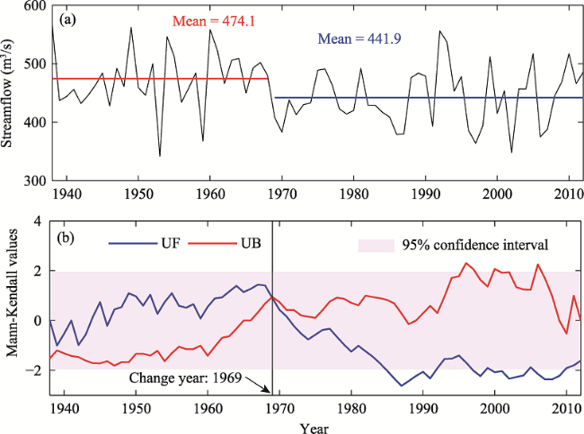
Figure 3 Annual streamflow (a) and Mann-Kendall mutation diagnosis (b) at the ZPP station during 1938-2012. UF and UB in (b) are statistics calculated by sequential and inverse streamflow records, respectively

4.2 Hydrological modelling and performance assessment

The datasets for the model setup, calibration, and verification procedures include meteorological forcing data, DEM data, land-use and soil data, and streamflow data. Firstly, by using the 90-m DEM data and a threshold of 100 km2, the UMR was split into 85 sub-basins, and geographic information for each sub-basin was extracted (Du et al., 2017). Then, the meteorological data were interpolated and corrected into each sub-basin using the IDW and their elevation information. The parameters related to soil types and land use for each sub-basin were calculated by area percentage. The observed and simulated daily streamflow processes are demonstrated as Figure 4. The NSE, PCC, PBIAS and RMSE are 0.73, 0.86, 1.51%, 177.35 and 0.72, 0.85, 5.94%, 183.46 during the calibration and verification period (Table 3). In general, the model showed satisfactory performance. Therefore, the calibrated parameters were considered to be suitable for simulating natural streamflow during the altered period.
Table 3 Model performance for daily discharge simulations at the ZPP station. Detailed description of these criteria can be found in Table 1
NSE PCC PBIAS RMSE
Calibration (1961‒1965) 0.73 0.86 ‒1.51% 177.35
Verification (1966‒1969) 0.72 0.85 5.94% 183.46
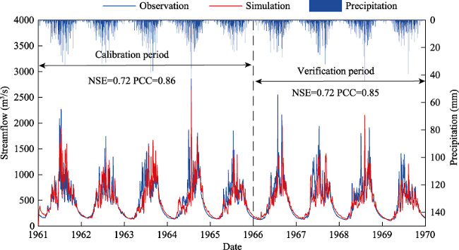
Figure 4 Observation and simulation of streamflow at the ZPP station during the calibration period (1961-1965) and verification period (1966-1969). (NSE: Nash-Sutcliffe efficiency; PCC: Pearson correlation coefficient)

4.3 Quantification of human and natural contributions to multi-dimensional hydrological alteration

Based on the observation and simulation of daily streamflow and Equations (9)-(11), we can obtain the total change rate of each IHA parameter in the altered period relative to that in the baseline period as well as the impacts from climate and human on the hydrological alterations, as shown in Figure 5a. For the total change in annual streamflow, which is similar to an earlier study (Hou et al., 2018). The water resource amount in the UMR decreased over the past half-century (1961-2012). In addition, for the multi-dimensional IHA parameters introduced in our study, 26 out of the 33 indicators also present a decreasing trend, and the change rates of all indicators are within the 40% range. From the perspective of climate change, 19 out of the 33 indicators present an increasing trend, and the remaining 14 indicators present a decreasing trend. On the basis of the impact of human activities, 22 of the 33 indicators express a decreasing trend, and the remaining 11 indicators express an increasing trend. Moreover, 31 of the 33 indicators present opposite trends, and only 2 indicators have the same trend.
Figure 6a displays the joint distribution of $\Delta {{I}_{c}}$ and $\Delta {{I}_{h}}$ for all groups of IHA parameters. In general, climate and human have opposite effects on the changes of IHA parameters, with scatter points falling in the second and fourth quadrants. Similarly, $\Delta {{I}_{c}}$ and $\Delta {{I}_{h}}$ in different groups of IHA parameters fall in different quadrants. Detailed results for each group of IHA parameters can be found in 6b-6f, and the corresponding values are shown in Table 4.
The IHA parameters in group 1 (Figure 6b) describe the annual and monthly discharge. With baseline as a reference, due to human contributions, the monthly and annual flows in all months show a decreasing trend (ranging from 1.7% to 27.4%), except in June and July, which indicates the increasing water demand during the dry season. However, the climate impact on the monthly average flow varies with seasons. The decreasing trend (ranging from 2% to 16.1%) is mainly concentrated in June, July and September. In other months, climate change plays a role in increasing streamflow. To a certain extent, these patterns reflect the climate effects on the seasonality of river discharge.
Figure 5 Relative changes (a) and relative contributions (b) for all IHA parameters induced by climate change versus those induced by human activities. The vertical dashed line indicates five groups.
In group 2 (Figure 6c), there are 11 parameters that display the degree and extent of annual extreme flows. All these parameters for the altered period present a decreasing trend. Human activities contribute to the occurrence of extremely low flow (ranging from 13.8% to 21%). Under the impact of climate change, QX1D, QX3D, QX7D, QX30D and QX90D show a decreasing trend (ranging from 5.5% to 16.3%), which may indicate the weakening trend of extremely heavy rainfall events in the UMR, and the corresponding extreme high discharge also decreased.
In group 3 (Figure 6d), there are two parameters to describe the time of occurrence of minimum discharge (Date min) and maximum discharge (Date max). From the perspective of human activities, Date min moved earlier by 4.8%, while Date max was postponed by 11.9%. This indicated that reservoir regulation and flood control can change the time of occurrence of minimum and maximum discharge. However, climate change, especially the temporal distribution of extreme precipitation, also affected the time of occurrence of extreme runoff.
According to the change rate in IHA indicators for the remaining two groups (Figure 6e and 6f), the Lo pulse #, the Hi pulse #, the Fall rate and Reversals show an increasing trend (ranging from 4.2% to 17.5%), while the Lo pulse L, the Hi pulse L, the Rise rate present a decreasing trend (ranging from 9.6% to 33.2%). Considering the single impact of climate change, the Hi pulse L and the Fall rate show an increasing trend, while other indicators show a decreasing trend. As for human activities, the Hi pulse L, the Rise and Fall rates show a downward trend, while other indicators show an upward trend. The construction and operation of hydropower stations changed the water level of the river, the high and low pulse and hydrological reversals change accordingly.
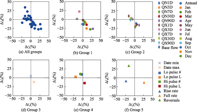
Figure 6 Joint distribution of the change rate for each group of IHA parameters induced by climate change $(\Delta {{I}_{c}})$ versus those induced by human activities $(\Delta {{I}_{h}}).$ The horizontal axis in the figure represents the change rate of IHA parameters caused by climate, and the vertical axis represents the change rate of IHA parameters caused by human.
Using the Mann-Whitney U test (M-W U test) (Nachar, 2008), we marked the significant change parameters in Table 4. Bold numbers show a significant difference in the altered period compared to that in the baseline period. Furthermore, according to Equations (12) and (13), we calculated the ${{\eta }_{c}}$ and ${{\eta }_{h}}$ to the change in IHA parameters (Figure 5b). Among these parameters, 23 out of the 33 indicators are dominated by the human impacts, including the monthly flow during the dry season, extremely low flow, time of occurrence of extreme flow, counts of low and high pulses, high-pulse duration and number of hydrological reversals. The other 10 indicators are dominated by the effects of climate change. Although a decreasing or increasing trend in a certain indicator may be dominated by the effects of a single factor, the influence of another factor cannot be ignored.
Table 4 IHA results, relative change and contributions calculated at the ZPP station. Bolded numbers indicate significant differences in the IHA indicators between two periods according to M-W U test at a significance level of 0.05. Mean (+) and mean (-) are the average values of increased and decreased parameters, respectively.
Index obsbp obsap simap obsnorm,bp obsnorm,ap simnorm,ap $\Delta I$(%) $\Delta {{I}_{c}}$(%) $\Delta {{I}_{h}}$(%) $\Delta {{\eta }_{c}}$(%) $\Delta {{\eta }_{h}}$(%)
Annual 452.1 418.6 456.4 0.478 0.352 0.494 -12.6 1.6 -14.2 10.1 89.9
January 163.0 159.1 182.9 0.213 0.198 0.292 -1.5 7.9 -9.4 45.7 54.3
February 143.2 140.5 153.3 0.235 0.221 0.284 -1.4 4.9 -6.3 43.8 56.3
March 164.2 154.6 189.8 0.306 0.266 0.413 -4.0 10.7 -14.7 42.1 57.9
April 246.7 257.4 397.6 0.185 0.205 0.464 2.0 27.9 -25.9 51.9 48.1
May 539.8 533.1 543.2 0.408 0.396 0.413 -1.2 0.5 -1.7 22.7 77.3
June 684.4 774.5 613.6 0.393 0.517 0.295 12.4 -9.8 22.2 30.6 69.4
July 914.2 755.7 735.9 0.506 0.363 0.345 -14.3 -16.1 1.8 89.9 10.1
August 689.3 602.1 716.3 0.425 0.325 0.456 -10.0 3.1 -13.1 19.1 80.9
September 754.1 640.6 738.9 0.568 0.417 0.548 -15.1 -2.0 -13.1 13.2 86.8
October 592.6 524.5 603.1 0.461 0.350 0.478 -11.1 1.7 -12.8 11.7 88.3
November 325.3 283.4 356.8 0.486 0.343 0.593 -14.3 10.7 -25.0 30.0 70.0
December 209.2 197.6 245.7 0.410 0.344 0.618 -6.6 20.8 -27.4 43.2 56.8
QN1D 136.9 112.6 138.7 0.596 0.400 0.610 -19.6 1.4 -21.0 6.3 93.8
QN3D 137.7 115.1 140.0 0.584 0.404 0.602 -18.0 1.8 -19.8 8.3 91.7
QN7D 138.9 118.6 142.5 0.566 0.409 0.593 -15.7 2.7 -18.4 12.8 87.2
QN30D 142.2 132.2 150.8 0.375 0.302 0.439 -7.3 6.4 -13.7 31.8 68.2
QN90D 158.3 152.2 180.2 0.346 0.312 0.470 -3.4 12.4 -15.8 44.0 56.0
QX1D 2014.3 1868.7 1657.0 0.509 0.442 0.346 -6.7 -16.3 9.6 62.9 37.1
QX3D 1711.8 1602.3 1538.0 0.450 0.393 0.359 -5.7 -9.1 3.4 72.8 27.2
QX7D 1411.2 1338.8 1329.7 0.425 0.376 0.369 -4.9 -5.6 0.7 88.9 11.1
QX30D 1091.5 1003.2 979.7 0.410 0.322 0.298 -8.8 -11.2 2.4 82.4 17.6
QX90D 891.4 811.7 821.20 0.558 0.424 0.440 -13.4 -11.8 -1.6 88.1 11.9
Base flow 0.29 0.27 0.3 0.531 0.460 0.570 -7.1 3.9 -11.0 26.2 73.8
Date min 56.7 72.5 56.5 0.077 0.124 0.076 4.7 -0.1 4.8 2.0 98.0
Date max 203.8 199.6 214.4 0.418 0.384 0.503 -3.4 8.5 -11.9 41.7 58.3
Lo pulse # 2.1 2.6 1.9 0.302 0.369 0.276 6.7 -2.6 9.3 21.8 78.2
Lo pulse L 57.9 34.3 30.8 0.423 0.250 0.225 -17.3 -19.8 2.5 88.8 11.2
Hi pulse # 11.3 12.0 10.2 0.431 0.473 0.367 4.2 -6.4 10.6 37.6 62.4
Hi pulse L 5.0 3.8 5.7 0.231 0.135 0.281 -9.6 5.0 -14.6 25.5 74.5
Rising rate 36.6 23.3 26.9 0.714 0.381 0.472 -33.3 -24.2 -9.1 72.7 27.3
Fall rate -18.1 -15.7 -13.2 0.415 0.545 0.676 13.0 26.1 -13.1 66.6 33.4
Reversals 107.8 129.5 87.6 0.289 0.463 0.126 17.4 -16.3 33.7 32.6 67.4
Mean (+) - - - - - - 8.6 8.3 9.2 41.4 58.6
Mean (-) - - - - - - -10.2 -10.8 -14.3

5 Discussion

5.1 The effects of climate change

Climate change mainly refers to variations in precipitation (P), temperature (T) and evapotranspiration (ET) in this study. To better attribute the climate impacts on the hydrological alterations, we calculated the changes in climate variables and streamflow at a monthly scale during the altered period with respect to their values during the baseline
period to explore whether the changes in these variables are consistent. From this, we can obtain the climatic factors that dominate the changes of monthly runoff.
The comparison between precipitation and streamflow (Figure 7a) illustrates a result similar to the patterns described above. The changes in IHA parameters are more closely related to climate change in the wet season (especially June to September). The increase or decrease in discharge is consistent with the changes in precipitation, but such consistency is declining in the dry season. The changes in temperature and the variation in discharge are almost irrelevant. Meanwhile, evapotranspiration is mainly controlled by precipitation, which shows good consistency. Therefore, the annual and monthly streamflows in the wet season are mainly affected by changes in precipitation.
For other IHA parameters, we try to cluster the types of IHA parameter changes using the correlation between them, and finally we can use precipitation changes to attribute changes in these factors. The results (Figure 7b) indicate that the mean monthly discharges in the dry season (especially from January to March) closely correlate with the QN1D, QN3D, QN7D, QN30D, QN90D, and the base flow index. Similarly, there are moderate correlations between the monthly discharge in the wet season (especially in June and July) and the QM1D, QM3D, QM7D, QM30D, QM90D. For the other IHA parameters, the correlation analysis did not express a significant relationship.
Based on Figure 7, we have gained a rough understanding of the multi-dimensional hydrological alterations from the perspective of climate change. Results conclude that the monthly and extreme indicators describing the river discharge in IHA are mainly affected by changes in precipitation, especially its seasonal distribution and magnitude. But for more complex indicators in IHA (e.g., high and low pulses and the number of hydrological reversals), which change frequently in river flow, more systematic analyses are required in future studies.
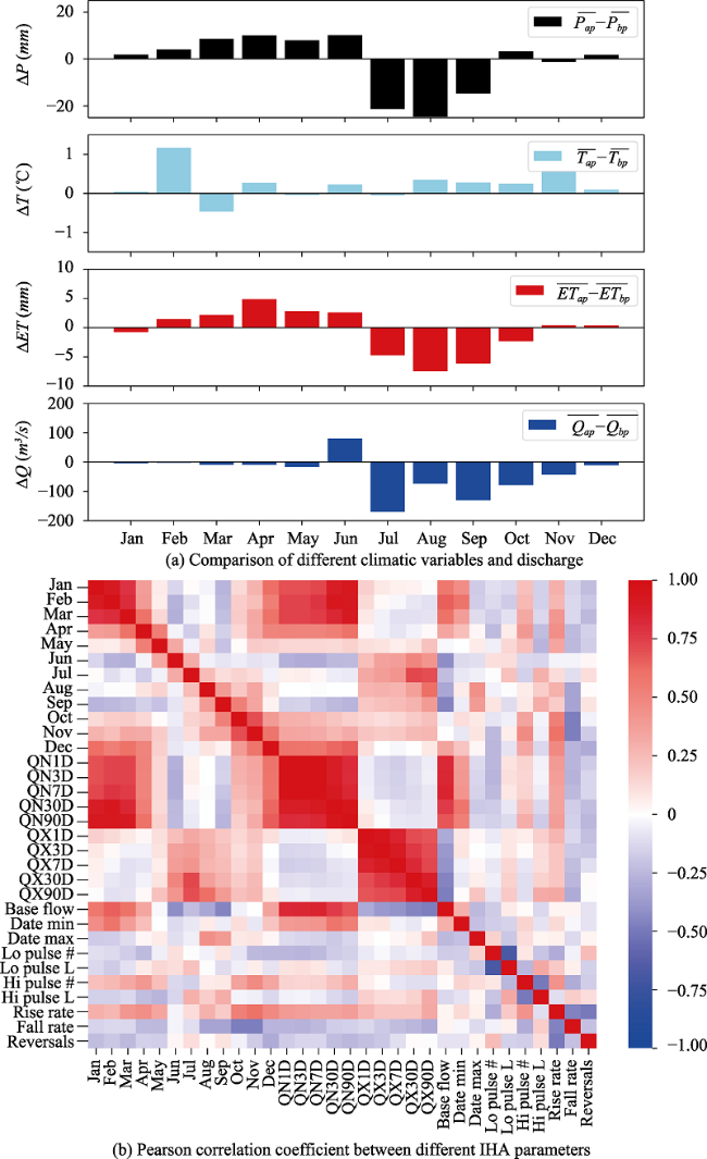
Figure 7 Comparison of different climatic variables and discharge (a) and Pearson correlation coefficient between different IHA parameters (b). In (a), $\overline{{{P}_{bp}}}$ and $\overline{{{P}_{ap}}}$ are the mean precipitation in the baseline and altered periods, respectively; $\overline{{{T}_{bp}}}$ and $\overline{{{T}_{ap}}}$ are the mean temperature in the baseline and altered periods, respectively; $\overline{E{{T}_{bp}}}$ and $\overline{E{{T}_{ap}}} $are the mean evapotranspiration in the baseline and altered periods, respectively; and $\overline{{{Q}_{bp}}}$ and $\overline{{{Q}_{ap}}}$ are the mean discharge in the baseline and altered periods, respectively.

5.2 The effects of human activities

Human impacts on the UMR mainly refer to dam construction and water withdrawal (Li et al., 2015). The different functions of reservoir projects include flood control, hydroelectric generation, water withdrawal and agricultural irrigation. Reservoirs with different functions have various impacts on hydrological process.
In the dry season, although the precipitation shows an increasing trend, the mean flow still shows a decreasing trend. This may be mainly attributed to more and more water withdrawal projects. According to statistical yearbook data (http://tjj.sc.gov.cn/), the population of Chengdu has increased by about 60% since the end of the 20th century, reaching 16 million in 2018. Moreover, the irrigated area reaches more than 1 million ha. In the wet season, reservoirs with flood regulation functions can reduce peak discharge. However, the changes related to the number of hydrological reversals and high- and low-flow may be attributed to reservoirs with the function of power generation. The types of hydropower stations on the UMR were mainly small-scale and rural hydropower stations, accounting for 82% of the total. In addition, there were 29 medium-scale hydropower stations and four large-scale hydropower stations (Li, 2014). According to the operation rules, both hydropower stations and flood control reservoirs needed to adjust the water level continuously, thus the number of hydrological reversals increases (Magilligan and Nislow, 2005). The construction and regulation of large reservoirs reduced flood peaks during high flow conditions and stored water to meet water demand in low flow conditions. (Graf, 2006; Gao et al., 2012; Räsänen et al., 2017).

5.3 Related impacts on river ecosystem

Although the streamflow analysis of the ZPP station did not show the phenomenon of zero-flow days, numerous studies showed that the construction of hydropower stations would cause the river reach to dry up and seriously damage the continuity of the river (Liang and Ding, 2004; Nakayama, 2011). The low flow trend of the ZPP station during the dry season also indicated that the river bed may dry up in the upper reaches, which damaged the integrity and posed a threat to the river ecosystem (Zhai et al., 2010; Wang et al., 2018). The decrease in high flow conditions may slow down the flow velocity and cause much sediment accumulation, which affects the chemical reaction of the water environment and ultimately threatens water safety (Chen et al., 2003; Yang et al., 2012). The magnitude of monthly discharge is closely related to water resource planning and management (Yang et al., 2008). The magnitude and duration of flow less than 25th percentile and those greater than the 75th percentile indicate the specific drought or flood conditions. Soil moisture, drought stress of plants and aquatic organic organisms will also be affected by the long-term drought of river flow (Graf, 2006). The decreased high- and low-pulse durations may reduce the hydraulic connectivity of river systems (Zhao et al. 2014). The rising rate, falling rate and number of hydrological reversals may be tied to amphibian migration (Wei et al., 2013; Chen et al., 2004).

6 Conclusions

We develop a DTVGM-IHA-based framework to evaluate the dual effects of climate and human on hydrological alterations in the UMR. The change rate and relative contribution are estimated by comparing the observed and simulated streamflow during the altered period, and possible reasons for these alterations are discussed. According to the results, we mainly conclude as follows:
(1) The DTVGM-IHA-based framework we proposed can meet the demand to assess multi-dimensional hydrological alterations. At the same time, it can be used to quantitatively estimate the climate and human contributions to these changes in the IHA parameters.
(2) Among the IHA parameters, 26 out of the 33 indicators present a decreasing trend (average -10.2%). The rising rate decreased significantly during the altered period. From the perspective of climate change, 19 out of the 33 indicators present an increasing trend (average 8.3%), and the remaining 14 indicators present a decreasing trend (average -10.8%). The average flow in April increased significantly due to climate change. As for human impacts, 22 of the 33 indicators show a decreasing trend (average -14.3%), and the remaining 11 indicators show an increasing trend (average 9.2%). The number of hydrological reversals changed most significantly due to human activities.
(3) Among the IHA parameters, the effects of human activities dominated the changes in hydrological alterations, with an average relative contribution rate of 58.6% and an average relative contribution rate of climate change of 41.4%. The scales of water withdrawal projects, the capabilities of the reservoir and hydroelectric plant are important factors that affect the degree of hydrological alteration. Changes in precipitation are the main forcing variable affecting hydrological alterations with respect to climate change.
(4) Practically speaking, the seasonal distribution of precipitation determines the seasonal distribution of river discharge. Extreme precipitation leads to more extreme river discharge. Meanwhile, reservoir regulation reduces the peak of river flow during the flood season and maintains the base flow in the dry season. The changes of low and high pulse, and the number of hydrological reversals bring more hydroelectric energy. Studying the changes in hydrological alterations is helpful to the integrated management of water resources, so as to achieve sustainable development.

Data availability

The gridded daily precipitation data and gauge-based meteorological data can be obtained from the National Climate Centre of the Chinese Meteorological Administration (CMA-NCC, http://data.cma.cn/data/cdcdetail/dataCode/SURF_CLI_CHN_PRE_DAY_GRID_0.5.html); Daily and monthly streamflow records for the ZPP hydrological station were collected from the Hydrological Yearbook of the Bureau of Hydrology, Yangtze River Water Resources Commission, in China; Digital elevation model (DEM) data with a spatial resolution of 3 arc-seconds were downloaded from NASA's Shuttle Radar Topography Mission website (SRTM, http://srtm.csi.cgiar.org/); The land use data were provided by the National Earth System Science Data Center, National Science & Technology Infrastructure of China (http://www.geodata.cn); The soil types data can be downloaded from the world soil database (Harmonized World Soil Database version 1.2, http://www.fao.org/soils-portal/soil-survey/soil-maps-and-databases/harmonized-world-soil-database-v12/en/).
[1]
Akbari S, Reddy M, 2019. Change detection and attribution of flow regime: A case study of Allegheny River catchment, PA (US). Science of The Total Environment, 662:192-204.

DOI

[2]
Chen S, Zhang G, Yang S, 2003. Temporal and spatial changes of suspended sediment concentration and resuspension in the Yangtze River estuary. Journal of Geographical Sciences, 13(4):498-506.

DOI

[3]
Chen Y, Li W, Chen Y et al., 2004. Physiological response of natural plants to the change of groundwater level in the lower reaches of Tarim River, Xinjiang. Progress in Natural Science, 14(11):975-983.

DOI

[4]
Dey P, Mishra A, 2017. Separating the impacts of climate change and human activities on streamflow: A review of methodologies and critical assumptions. Journal of Hydrology, 548:278-290.

DOI

[5]
Donat M, Lowry A, Alexander L et al., 2016. More extreme precipitation in the world's dry and wet regions. Nature Climate Change, 6(5):508-513.

DOI

[6]
Du C, Ye A, Gan Y et al., 2017. Drainage network extraction from a high-resolution DEM using parallel programming in the NET framework. Journal of Hydrology, 555:506-517.

DOI

[7]
Gao B, Yang D, Zhao T et al., 2002. Changes in the eco-flow metrics of the Upper Yangtze River from 1961 to 2008. Journal of Hydrology, 448/449:30-38.

DOI

[8]
Graf W, 2006. Downstream hydrologic and geomorphic effects of large dams on American rivers. Geomorphology, 79(3):336-360.

DOI

[9]
Gupta H, Sorooshian S, Yapo P, 1999. Status of automatic calibration for hydrologic models: Comparison with multilevel expert calibration. Journal of Hydrologic Engineering, 4(2):135-143.

DOI

[10]
Hou J, Ye A, You J et al., 2018. An estimate of human and natural contributions to changes in water resources in the upper reaches of the Min River. Science of The Total Environment, 635:901-912.

DOI

[11]
Jiang C, Zhang L, Tang Z et al., 2017. Multi-temporal scale changes of streamflow and sediment discharge in the headwaters of Yellow River and Yangtze River on the Tibetan Plateau, China. Ecological Engineering, 102:240-254.

DOI

[12]
Kendall M, Gibbons J, 1948. Rank Correlation Methods. 5th ed. London, UK: Edward Arnold, 320.

[13]
Kundzewicz Z, 2008. Climate change impacts on the hydrological cycle. Ecohydrology & Hydrobiology, 8(2-4):195-203.

[14]
Li M, 2014. Cumulative influence of cascade hydropower development on runoff in upper reaches of Min River[D]. Chengdu: Chengdu University of Technology. (in Chinese)

[15]
Li M, Fu B, Wang Y et al., 2015. Characteristics and spatial patterns of hydropower development in the upper Min River basin. Resources and Environment in the Yangtze Basin, 24(1):74-80. (in Chinese)

[16]
Li Z, Li X, Xu Z, 2010. Impacts of water conservancy and soil conservation measures on annual runoff in the Chaohe River Basin during 1961-2005. Journal of Geographical Sciences, 20(6):947-960.

DOI

[17]
Liang G, Ding S, 2004. Impacts of human activity and natural change on the wetland landscape pattern along the Yellow River in Henan Province. Journal of Geographical Sciences, 14(3):339-348.

DOI

[18]
Liu X, Liu C, Luo Y et al., 2012. Dramatic decrease in streamflow from the headwater source in the central route of China's water diversion project: Climatic variation or human influence? Journal of Geophysical Research:Atmospheres, 117:D06113.

[19]
Liu X, Shen Y, Guo Y et al., 2015. Modelling demand/supply of water resources in the arid region of northwestern China during the late 1980s to 2010. Journal of Geographical Sciences, 25(5):573-591.

DOI

[20]
Lu E, Zhao W, Zou X et al., 2017. Temporal-spatial monitoring of an extreme precipitation event: Determining simultaneously the time period it lasts and the geographic region it affects. Journal of Climate, 30(16):6123-6132.

DOI

[21]
Lu W, Lei H, Yang D et al., 2018. Quantifying the impacts of small dam construction on hydrological alterations in the Jiulong River basin of Southeast China. Journal of Hydrology, 567:382-392.

DOI

[22]
Luca P, Messori G, Wilby R et al., 2019. Concurrent wet and dry hydrological extremes at the global scale. Earth System Dynamics, 11(1):251-266.

DOI

[23]
Ma F, Ye A, Gong W et al., 2014. An estimate of human and natural contributions to flood changes of the Huai River. Global and Planetary Change, 119(4):39-50.

DOI

[24]
Ma H, Yang D, Tan S et al., 2010. Impact of climate variability and human activities on streamflow decrease in the Miyun Reservoir catchment. Journal of Hydrology, 389(3/4):317-324.

DOI

[25]
Magilligan F, Nislow K, 2005. Changes in hydrologic regime by dams. Geomorphology, 71(1):61-78.

DOI

[26]
Mann H, 1945. Nonparametric test against trend. Econometrica, 13(3):245-259.

DOI

[27]
Mittal N, Bhave A, Mishra A et al., 2016. Impact of human intervention and climate change on natural flow regime. Water Resources Management, 30(2):685-699.

DOI

[28]
Nachar N, 2008. The Mann-Whitney U: A test for assessing whether two independent samples come from the same distribution. Tutorials in Quantitative Methods for Psychology, 4(1):13-20.

DOI

[29]
Nakayama T, 2011. Simulation of the effect of irrigation on the hydrologic cycle in the highly cultivated Yellow River Basin. Agricultural and Forest Meteorology, 151(3):314-327.

DOI

[30]
Nash J, Sutcliffe J, 1970. River flow forecasting through conceptual models: Part 1 A discussion of principles. Journal of Hydrology, 10(3):282-290.

DOI

[31]
Räsänen T, Someth P, Lauri H et al., 2017. Observed river discharge changes due to hydropower operations in the Upper Mekong Basin. Journal of Hydrology, 545:28-41.

DOI

[32]
Richter B, Baumgartner J, Powell J et al., 1996. A method for assessing hydrologic alteration within ecosystems. Conservation Biology, 10(4):1163-1174.

DOI

[33]
Shepard D, 1984. Computer mapping:The SYMAP interpolation algorithm. In: Spatial Statistics and Models. Dordrecht: Springer,133-145.

[34]
Shrestha S, Htut A, 2016. Land use and climate change impacts on the hydrology of the Bago River Basin, Myanmar. Environmental Modelling & Assessment, 21(6):819-833.

[35]
Sun Q, Miao C, Duan Q, 2015. Projected changes in temperature and precipitation in ten river basins over China in 21st century. International Journal of Climatology, 35(6):1125-1141.

DOI

[36]
Talukdar S, Pal S, 2019. Effects of damming on the hydrological regime of Punarbhaba River basin wetlands. Ecological Engineering, 135:61-74.

DOI

[37]
Wan Z, Chen X et al., 2020. Streamflow reconstruction and variation characteristic analysis of the Ganjiang River in China for the past 515 years. Sustainability, 12(3):1168.

DOI

[38]
Wang G, Xia J, Chen J, 2009. Quantification of effects of climate variations and human activities on runoff by a monthly water balance model: A case study of the Chaobai River basin in northern China. Water Resources Research, 45:W00A11.

[39]
Wang G, Xia J, Tan G et al., 2002. A research on distributed time variant gain model: A case study on Chaohe River Basin. Progress in Geography, 21(6):573-582. (in Chinese)

[40]
Wang J, Dai Z, Mei X et al., 2018. Immediately downstream effects of Three Gorges Dam on channel sandbars morphodynamics between Yichang-Chenglingji Reach of the Changjiang River, China. Journal of Geographical Sciences, 28(5):629-646.

DOI

[41]
Wang X, 2014. Advances in separating effects of climate variability and human activities on stream discharge: An overview. Advances in Water Resources, 71:209-218.

DOI

[42]
Wang X, Yang T, Wortmann M et al., 2017. Analysis of multi-dimensional hydrological alterations under climate change for four major river basins in different climate zones. Climatic Change, 141(3):483-498.

DOI

[43]
Wei W, Shi P, Zhou J et al., 2013. Environmental suitability evaluation for human settlements in an arid inland river basin: A case study of the Shiyang River Basin. Journal of Geographical Sciences, 23(2):331-343.

DOI

[44]
Wu J, Miao C, Zhang X et al., 2017. Detecting the quantitative hydrological response to changes in climate and human activities. Science of The Total Environment, 586:328-337.

DOI

[45]
Wu J, Miao C, Wang Y et al., 2016. Contribution analysis of the long-term changes in seasonal runoff on the Loess Plateau, China, using eight Budyko-based methods. Journal of Hydrology, 545:263-275.

DOI

[46]
Wu X, Wang Z, Zhou X et al., 2016. Observed changes in precipitation extremes across 11 basins in China during 1961-2013. International Journal of Climatology, 36(8):2866-2885.

DOI

[47]
Xia J, 1991. Identification of a constrained nonlinear hydrological system described by volterra functional series. Water Resources Research, 27(9):2415-2420.

DOI

[48]
Xia J, Wang G, Lv A et al., 2003. A research on distributed time variant gain modelling. Acta Geographica Sinica, 58(5):789-796. (in Chinese)

[49]
Xia J, Wang G, Tan G et al., 2005. Development of distributed time-variant gain model for nonlinear hydrological systems. Science in China Series D:Earth Sciences, 48(6):713-723.

[50]
Xin Z, Li Y, Zhang L et al., 2019. Quantifying the relative contribution of climate and human impacts on seasonal streamflow. Journal of Hydrology, 574:936-945.

DOI

[51]
Xu C, Wang J, Li Q, 2018: A new method for temperature spatial interpolation based on sparse historical stations. Journal of Climate, 31:1757-1770.

DOI

[52]
Yang S, Milliman J, Li P et al., 2011. 50,000 dams later: Erosion of the Yangtze River and its delta. Global and Planetary Change, 75(1/2):14-20.

DOI

[53]
Yang T, Cui T, Xu C et al., 2017. Development of a new IHA method for impact assessment of climate change on flow regime. Global & Planetary Change, 156(9):68-79.

[54]
Yang T, Zhang Q, Chen Y et al., 2008. A spatial assessment of hydrologic alteration caused by dam construction in the middle and lower Yellow River, China. Hydrological Processes, 22(18):3829-3843.

DOI

[55]
Yang Z, Yan Y, Liu Q, 2012. Assessment of the flow regime alterations in the Lower Yellow River, China. Ecological Informatics, 10(7):56-64.

DOI

[56]
Ye A, Duan Q, Chu W et al., 2014. The impact of the south-north water transfer project (CTP)'s central route on groundwater table in the Hai River Basin, North China. Hydrological Processes, 28(23):5755-5768.

DOI

[57]
Ye A, Duan Q, Schaake J et al., 2015. Post-processing of ensemble low flow forecasts. Hydrological Processes, 29:2438-2453.

DOI

[58]
Ye A, Duan Q, Zeng H et al., 2010. A distributed time-variant gain hydrological model based on remote sensing. Journal of Resources and Ecology, 1(3):222-230.

[59]
Ye A, Duan Q, Zhan C et al., 2013. Improving kinematic wave routing scheme in Community Land Model. Hydrology Research, 44(5):886-903.

DOI

[60]
Ye A, Xia J, Wang G, 2006. Dynamic network-based distributed kinematic wave affluent model. Yellow River, 28(2):26-29. (in Chinese)

[61]
Zhai H, Cui B, Hu B et al., 2010. Prediction of river ecological integrity after cascade hydropower dam construction on the mainstream of rivers in Longitudinal Range-Gorge Region (LRGR), China. Ecological Engineering, 36(4):361-372.

DOI

[62]
Zhang M, Wei X, Sun P et al., 2012. The effect of forest harvesting and climatic variability on runoff in a large watershed: The case study in the Upper Min River of Yangtze River Basin. Journal of Hydrology, 464:1-11.

[63]
Zhao G, Tian P, Mu X et al., 2014. Quantifying the impact of climate variability and human activities on streamflow in the middle reaches of the Yellow River Basin, China. Journal of Hydrology, 519:387-398.

DOI

[64]
Zhao L, Peng Q, Li C et al., 2014. Analysis of eco-hydrological alteration of upper Yangtze mainstream sections in the nature reserves for rare and endemic fishes. Journal of Hydroelectric Engineering, 33(3):106-111. (in Chinese)

[65]
Zhao Q, Liu S, Deng L et al., 2012. The effects of dam construction and precipitation variability on hydrologic alteration in the Lancang River Basin of Southwest China. Stochastic Environmental Research and Risk Assessment, 26(7):993-1011.

DOI

[66]
Zhou B, Wen, Q, Xu Y et al., 2014. Projected changes in temperature and precipitation extremes in China by the CMIP5 multi-model ensembles. Journal of Climate, 27(17):6591-6611.

DOI

Outlines

/