Research Articles

Monthly calibration and optimization of Ångström-Prescott equation coefficients for comprehensive agricultural divisions in China

  • XIA Xingsheng , 1, 2 ,
  • PAN Yaozhong 1, 2 ,
  • ZHU Xiufang , 1, 3, * ,
  • ZHANG Jinshui 1, 3
Expand
  • 1. State Key Laboratory of Remote Sensing Science, Jointly Sponsored by Beijing Normal University and Institute of Remote Sensing and Digital Earth of Chinese Academy of Sciences, Beijing 100875, China
  • 2. Academy of Plateau Science and Sustainability, Qinghai Normal University, Xining 810016, China
  • 3. Institute of Remote Sensing Science and Engineering, Faculty of Geographical Science, Beijing Normal University, Beijing 100875, China
* Zhu Xiufang, PhD and Associate Professor, E-mail:

Xia Xingsheng, PhD and Instructor, specialized in crop water requirements research. E-mail:

Received date: 2021-02-20

  Accepted date: 2021-04-28

  Online published: 2021-09-25

Supported by

National High Resolution Earth Observation System (the Civil Part) Technology Projects of China

Local Scientific & Technological Development Projects of Qinghai Guided by Central Government of China

Disaster Research Foundation of PICC P&C(2017D24-03)

Copyright

Copyright reserved © 2021.

Abstract

Ångström-Prescott equation (AP) is the algorithm recommended by the Food and Agriculture Organization (FAO) of the United Nations for calculating the surface solar radiation (Rs) to support the estimation of crop evapotranspiration. Thus, the as and bs coefficients in the AP are vital. This study aims to obtain coefficients as and bs in the AP, which are optimized for China’s comprehensive agricultural divisions. The average monthly solar radiation and relative sunshine duration data at 121 stations from 1957-2016 were collected. Using data from 1957 to 2010, we calculated the monthly as and bs coefficients for each subregion by least-squares regression. Then, taking the observation values of Rs from 2011 to 2016 as the true values, we estimated and compared the relative accuracy of Rs calculated using the regression values of coefficients as and bs and that calculated with the FAO recommended coefficients. The monthly coefficients, as and bs, of each subregion are significantly different, both temporally and spatially, from the FAO recommended coefficients. The relative error range (0-54%) of Rs calculated via the regression values of the as and bs coefficients is better than the relative error range (0-77%) of Rs calculated using the FAO suggested coefficients. The station-mean relative error was reduced by 1% to 6%. However, the regression values of the as and bs coefficients performed worse in certain months and agricultural subregions during verification. Therefore, we selected the as and bs coefficients with the minimum Rs estimation error as the final coefficients and constructed a coefficient recommendation table for 36 agricultural production and management subregions in China. These coefficient recommendations enrich the case study of coefficient calibration for the AP in China and can improve the accuracy of calculating Rs and crop evapotranspiration based on existing data.

Cite this article

XIA Xingsheng , PAN Yaozhong , ZHU Xiufang , ZHANG Jinshui . Monthly calibration and optimization of Ångström-Prescott equation coefficients for comprehensive agricultural divisions in China[J]. Journal of Geographical Sciences, 2021 , 31(7) : 997 -1014 . DOI: 10.1007/s11442-021-1882-4

1 Introduction

Solar radiation is the most important energy source in biological, physical, and chemical processes on the surface of Earth (Liu et al., 2014), as well as one of the sources of green energy that support the sustainable development of human society (Paulescu et al., 2016). Accurate measurement or estimation of solar radiation (Rs) with high spatial and temporal resolutions is of great significance for the study of changes in the surface environment, food safety production, and the implementation of solar energy projects (Qin et al., 2011; Pan et al., 2013; Paulescu et al., 2016). Numerous countries have also established Rs observation systems for this purpose (Paulescu et al., 2013). However, due to high investment and maintenance costs, the density of stations that can continuously perform Rs observation is too low (Paulescu et al., 2013). In China, for example, there are more than 2400 national meteorological stations, but only data from 130 stations belong to the radiation dataset released by the China Meteorological Data Service Center (CMDC). Therefore, numerous studies have developed models to estimate Rs, which are more cost-effective than observations of Rs (Paulescu et al., 2016). At present, the developed models include the remote sensing inversion model (Olseth and Skartveit, 2001), stochastic simulation model (Richardson, 1981), empirical model (Ångström, 1924; Prescott, 1940; Li et al., 2010), and machine learning model (Chen et al., 2011). Among them, empirical models based on sunshine duration and temperature are widely popular because of their simplicity and ease of use (Li et al., 2012a), where the results of the Ångström-Prescott equation (AP) yield the best performance (Iziomon and Mayer, 2002; Almorox and Hontoria, 2004; Trnka et al., 2005; Zhang et al., 2018). In addition, in the Crop Evapotranspiration-Guidelines for Computing Crop Water Requirements (FAO 56) (Allen et al., 1998), published by the Food and Agriculture Organization (FAO) of the United Nations in 1998, the Penman-Monteith equation (PM) is recommended as a scheme to calculate the true value for reference crop evapotranspiration (ET0). In this scheme, the AP was also suggested to calculate missing Rs values to support the PM in a specific study or application area. Therefore, the as and bs coefficients are important to accurately estimate Rs in the AP.
Existing studies use two main methods to determine coefficients as and bs. In areas without measured solar radiation data, previous studies have directly used the recommended values, i.e., as = 0.25 and bs = 0.50 for the Ångström and FAO 56 (Ångström, 1924; Allen et al., 1998; Du et al., 2003; Zhao et al., 2008; Mai et al., 2012; Ma et al., 2013; Cui, 2014; Lu et al., 2016). However, the spatial and temporal differences in atmospheric components exist objectively due to long-term climate and short-term seasonal changes at the surface, such that the disadvantages of globally fixed as and bs coefficients are evident. In areas where portions of measured solar radiation data are available, the measured data are often used to correct the as and bs coefficients; the corrected coefficients can better reflect the influence that atmospheric conditions have on Rs (Wen, 1964; Ju et al., 2005; Yang et al., 2009). Therefore, the coefficient correction of the AP has attracted extensive attention.
Some studies have introduced terrain (Liu et al., 2017), air temperature (Ojosu and Komolafe, 1987), relative humidity (Ododo et al., 1995), water vapor pressure (Liu et al., 2017), and other geographical factors (Glover and McCulloch, 1958; Gopinathan, 1988; Zhou et al., 2005) or key meteorological factors (Halouani et al., 1993) for AP coefficient correction based on the analysis of the factors that influence Rs. These studies have proven that the AP coefficient is characterized by large differences between regions owing to the influence of geographical (such as altitude) and climate/weather (such as cloud cover) factors, recommending corrected coefficients based on their hypothesis and the AP correction scheme (Liu et al., 2019). However, other studies (Ögelman et al., 1984; Akinoğlu and Ecevit, 1990; Ertekin and Yaldiz, 2000; Iziomon and Mayer, 2002; Almorox and Hontoria, 2004; Yorukoglu and Celik, 2006) have pointed out that, due to the correlation between different variables, a complex model with other factors does not show evident advantages compared with the original AP (Liu et al., 2009a; Liu et al., 2010). Therefore, numerous studies continue to adopt simple and feasible traditional regression correction methods (Liu et al., 2010). For example, in China, Yin et al. (2008) used data from 81 meteorological stations from 1971 to 2000 to analyze and determine that when as and bs were 0.20 and 0.79, respectively, nationwide, the Rs error for the 30 remaining verification stations was the smallest. Hu et al. (2010) divided China into seven regions, analyzing and discussing the values of as and bs in different regions based on 20 years of observation data. At a small regional scale, Peng et al. (2006), Liu et al. (2009b), Li et al. (2012b), Cao et al. (2014) and Yuan et al. (2018) discussed the as and bs correction values in the Yellow River Basin, Anhui, Yunnan, Jiangsu, and other regions. Although these studies show that the Rs estimated by the as and bs values suggested by the FAO is larger than the observed Rs, as and bs values, corrected using the observation data, can effectively improve the precision of the estimated Rs. This improvement, however, is mostly concentrated on the time scale of a year, ignoring the fact that the as and bs values may change over time within a year (Paulescu et al., 2016). Data analysis by Liu et al. (2010) at 20 observation stations in northern China showed that fixed as and bs coefficients for the AP can improve the estimation accuracy of Rs, reduce unnecessary complexity in the model, and are convenient for wide application. However, China is located in a typical monsoon climate zone, such that the solar radiation reaching the surface changes significantly throughout a year. In certain regions, unified as and bs values may lead to seasonal error in the Rs estimations (Xia et al., 2020a). For example, Li et al. (2012a), based on observational data from 15 stations in the Yangtze River Basin, showed that the as and bs coefficients change with time over a year, where the coefficients obtained on a shorter time scale can be used to estimate the Rs at a longer time scale. In addition, if the Rs estimated by the fixed as and bs coefficients in a specific year is directly applied to the calculation of ET0, error transfer will also affect the calculation results for the ET0 (Xia et al., 2020a). Therefore, the spatio-temporal changes in the as and bs values throughout the country require further discussion.
Based on the above analysis, the purpose of this study is to obtain the corrected coefficients of the AP at a specific spatio-temporal scale in China. Considering the natural geographical background of agricultural production, such as the type of agricultural region and planting system based on the diverse characteristics of water and heat combinations in China, agricultural production management, and comprehensive agricultural regionalization, the comprehensive agricultural divisions were selected as the framework, including nine primary agricultural regions (Regions A-I) and 38 subregions as division benchmarks. We used the least-squares regression method to calculate the correction coefficients for the AP for every month in every subregion. Based on this, we discuss the characteristics of the as and bs coefficients in each subregion. Finally, by comparing the application errors of our values and the FAO recommended values, we provide the optimal correction coefficients as and bs for every month to obtain a parameter basis for the calculation of high precision Rs values.

2 Data and preprocessing

According to the AP (1), the data used in this study include the following: 1) the total monthly effective Rs data from 1957 to 2016 from the Dataset of Monthly Values of Radiation Data from Chinese Surface Stations (a total of 130 stations), in which data before 2011 were used to correct the as and bs coefficients while data from 2011 to 2016 were used to verify the accuracy of the estimated Rs calculated using the corrected as and bs coefficients; 2) the average daily relative sunshine duration of each month from 1957 to 2016 from the Dataset of Monthly Values of Climate Data from Chinese Surface Stations (a total of 756 stations), i.e., the input data for the AP; 3) longitude and latitude data for each station for the calculation of the Ra. The above three datasets are from the CMDC (http://data.cma.cn/) and 4) The Comprehensive Agricultural Regionalization Map of China (Figure 1), issued by the National Agriculture Commission, which served as the basis for agricultural divisions in this study. We can calculate the Rs as follows:
${{R}_{s}}=\left( {{a}_{s}}+{{b}_{s}}\frac{n}{N} \right){{R}_{a}}$
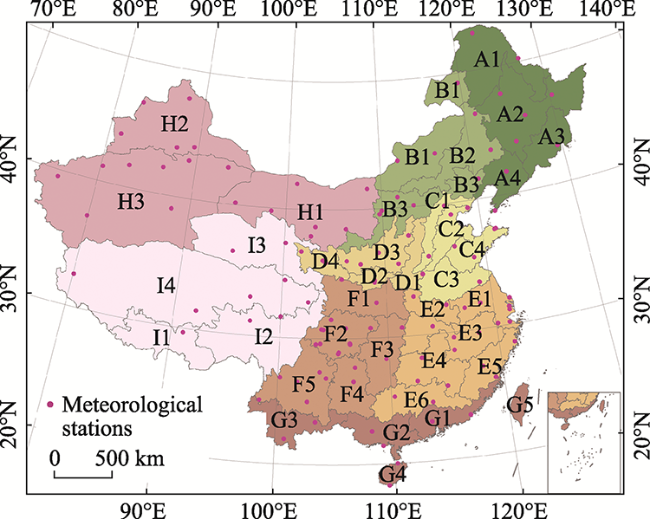
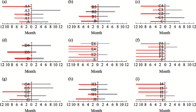
Figure 1 Comprehensive agricultural divisions and data station locations (A. Northeastern China. A1: Hinggan; A2: Songnen and Sanjiang Plain; A3: Changbai Mountains; A4: Liaoning Plain. B. Inner Mongolia and Regions along the Great Wall. B1: Northern Inner Mongolia; B2: Central and Southern Inner Mongolia; B3: Regions along the Great Wall. C. Huang-Huai-Hai. C1: Piedmont at the foot of the Yanshan and Taihang Mountains; C2: Low-lying plain regions of Hebei, Shandong, and Henan; C3: Huang-huai Plain; C4: Hilly region of Shandong. D. Loess Plateau. D1: Hilly region of Western Henan and Eastern Shanxi; D2: Fenhe and Weihe valleys; D3: Hilly loess region of Shanxi, Shaanxi, and Gansu; D4: Hilly region of Central Gansu and Eastern Qinghai. E. Middle and Lower Reaches of the Yangtze River. E1: Lower Yangtze Plain; E2: Mountainous regions of Henan, Hubei, and Anhui; E3: Plains in the Middle Reaches of the Yangtze River; E4: Hilly regions south of the Yangtze River; E5: Hilly region of Zhejiang and Fujian; E6: Hilly regions of Nanling. F. Southwestern China. F1: Qinling and Daba Mountains; F2: Sichuan Basin; F3: Border between Sichuan, Hubei, Hunan, and Guizhou; F4: Guizhou and Guangxi plateaus; F5: Sichuan and Yunnan plateaus. G. Southern China. G1: Southern Fujian and Central Guangdong; G2: Western Guangdong and Southern Guangxi; G3: Southern Yunnan; G4: Hainan and South China Sea Islands; G5: Taiwan. H. Gansu and Xinjiang. H1: Border between Inner Mongolia, Ningxia, and Gansu; H2: Northern Xinjiang; H3: Southern Xinjiang. I. Tibet. I1: Southern Tibet; I2: Border between Sichuan and Tibet; I3: Border between Qinghai and Gansu; and I4: High cold region of Tibet).
where Rs is the solar radiation (MJ m-2 day-1); n is the actual duration of sunshine (h); N is the maximum possible duration of sunshine or daylight (h); n/N is the relative sunshine duration; Ra is the extraterrestrial radiation (MJ m-2 day-1); as is a regression constant expressing the fraction of extraterrestrial radiation that reaches the Earth’s surface on overcast days (n = 0); and as + bs is the fraction of extraterrestrial radiation that reaches the Earth’s surface on clear days (n = N).
Data preprocessing included the following steps. 1) The total monthly Rs (MJ m-2 month-1) was converted to a daily average (MJ m-2 day-1) and associated with the relative sunshine duration by station number. 2) The average daily Ra of each month was obtained according to the procedure for Ra for daily periods recommended by FAO 56 (Allen et al., 1998). 3) Theoretically, due to the existence of the atmosphere, the solar radiation observed on the ground must be lower than the Ra. However, in actual observations, the solar radiation observed on the ground at certain stations was higher than the Ra due to loss of and damage to the instruments and equipment or errors associated with observation operation, which were eliminated in this study. Finally, the number of stations with valid data throughout the land extent of China, obtained via station association and data screening, was 121 (Figure 1). 4) For agricultural regionalization, based on the latitude and longitude in Figure 1 and the vector data at the 1:250,000 administrative regionalization in China, the regional vector data required for this study were obtained after spatial correction under the Albers projection.

3 Coefficient correction process

The coefficient correction process for the AP mainly includes four parts: data preprocessing, regression calculation of the as and bs coefficients, verification of the Rs estimation results, and determination of the monthly as and bs coefficients in each subregion. The details are as follows.
1) Data preprocessing. This process has been explained in the preceding section and is not repeated here.
2) Regression calculation of the as and bs coefficients. Based on the pre-processed observed Rs and relative sunshine duration data before 2011, the least-squares regression method was adopted to estimate the as and bs coefficients on a station-by-station basis. Then, the average values of the as and bs coefficients at the stations in each subregion were obtained.
3) Verification of the estimated Rs. According to the AP, as well as based on the relative sunshine duration observations and Ra from 2011-2016, using the subregions’ as and bs coefficients from step 2 and FAO recommended as and bs coefficient values, two groups of Rs values were calculated. The relative error of the two estimated Rs values was compared to verify the reliability and applicability of the regression as and bs coefficients taking the Rs observation data from 2011-2016 as the true values.
4) Determination of the monthly as and bs coefficients in each subregion. The Rs errors estimated by the as and bs coefficients obtained using the least-squares regression and those suggested by the FAO were compared month-by-month. The values of the as and bs coefficients with smaller Rs estimation errors were selected as the final optimal coefficients.

4 Results and analysis

4.1 Regression results for the AP coefficients

Figure 2 shows the results for the monthly station average as and bs coefficients of each agricultural subregion based on the least-squares regression. Overall, the regression values of the as and bs coefficients vary in different months in the same agricultural subregion, where there are notable differences in the same month in different agricultural subregions.
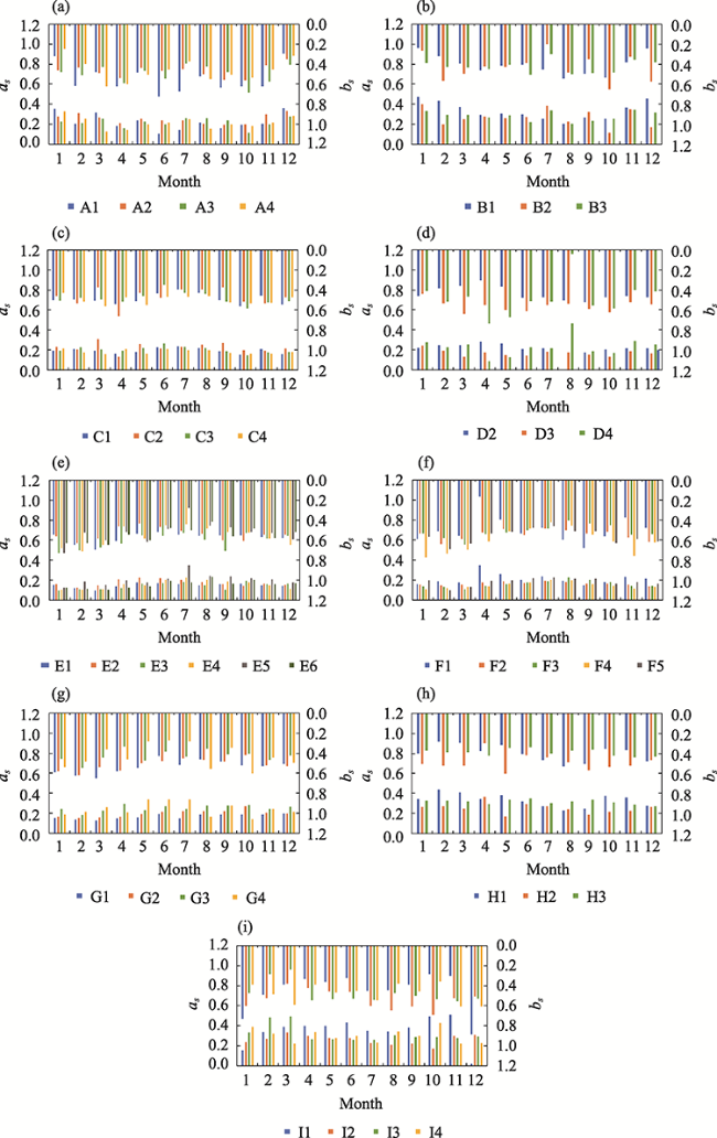
Figure 2 The mean monthly station value of the as and bs coefficients calculated via the least-squares regression for each subregion: a. A1-A4, b. B1-B3, c. C1-C4, d. D2-D4, e. E1-E6, f. F1-F5, g. G1-G4, h. H1-H3, and i. I1-I4
The overall performance in Northeastern China (Region A) shows relative stability for coefficient as while the volatility of bs is relatively large. For the coefficient of as, the A1 region was higher during the winter and spring months and lower during the summer and autumn months. The other three regions showed a gradual decrease from January to less than 0.25, followed by an increase to ~0.25 from May to August, and then an increase exceeding 0.25 in November and December after a slight decrease in September and October. For coefficient bs, A1 is the special subregion, which exhibits intermittent increases and decreases. The maximum value is more than 0.7, the minimum value is less than 0.3, and for half of the months, the values are more than 0.6. The bs values of the other three subregions are lower in the winter and summer months and higher in the spring and autumn months.
For Inner Mongolia and the Regions along the Great Wall (Region B), the as and bs coefficients in each subregion have no evident differences in April, May, August, and November, as well as relatively evident differences between each subregion for the other months. Even individual months exhibit relative minimum or maximum values, such as B1 and B3 in the winter months, where coefficient as is larger. Furthermore, B2 has a relatively small as coefficient in October, December, and February, with a corresponding larger bs coefficient while in June, the values of the as and bs coefficients are the opposite.
Huang-Huai-Hai (Region C), except for C2 in March and September, yields a stable as coefficient for all time periods at approximately 0.2. In summer, this value was slightly higher than 0.2 but less than 0.25, whereas in the other months, this value was slightly less than 0.2. For coefficient bs, in addition to the abnormally high value (0.66) for C2 in April, the overall performance from autumn to early spring in each subregion was relatively stable. The values for the summer months were significantly reduced, but there is still a difference for each subregion. For example, in March, May, August, September, October, and December, the bs coefficients for C2 were smaller than that for other subregions.
For the Loess Plateau (Region D), data for D1 were not available because there is no valid data station. The as and bs coefficients for D2, D3, and D4 were significantly different from each other. In D2, coefficient as was higher than 0.2 in the winter and spring months, at approximately 0.2 in the summer months and slightly lower than 0.2 in the autumn months. The bs coefficient exhibits a “big wave” pattern. The bs is high in the summer and autumn months, whereas it is low in the spring months and slightly high during the other months. In D3, the as coefficient is stable, below 0.2, in the other months, except for 0.24 in January, and it has the smallest value of 0.13 in March and October. Coefficient bs, with a large value and volatility, exhibits the opposite trend to as. In D4, the as coefficient was abnormally high in August while the corresponding bs coefficient was abnormally low. The as in January, February, March, June, July, November, and December were slightly higher while the corresponding bs value was relatively low. This was the opposite case during the other months. Overall, the bs coefficients in D4 were at a higher range.
For the Middle and Lower Reaches of the Yangtze River (Region E), except for E3 and E5, the value of coefficient as was stable and low while the value of coefficient bs was, overall, stable and high. Here, the as was lower in the winter and spring months, but higher in the summer and autumn months. The bs coefficient exhibited an opposite trend. The difference between the subregions is also notable. For example, as in E5 was significantly higher than that in other regions while as in E2 was significantly higher than that in other subregions in April, May, and June. Furthermore, bs surpassed a value of 0.5 in nearly all subregions, except during the summer months, with E3 peaking at 0.73 in January.
For Southwestern China (Region F), in F1, the as coefficient first increased and then decreased with volatility while the corresponding bs value showed the opposite trend. Second, in F4, the bs coefficient showed a significant change from 0.42 to 0.77, first decreasing and then increasing. The corresponding as value exhibited an opposite trend, but with a smaller range, i.e., between 0.1 and 0.2. The variation in the other subregions was similar to that of F4, but the variation range was smaller and more stable than that of F4.
In comparison, Southern China (Region G) was the most stable region in the time series. More specifically, as was higher in G4 in May, June, and July while other months showed slight fluctuations. Other subregions had slightly higher values in the second half of the year than at the beginning of the year. The corresponding bs values were the opposite. The as values for the subregions can be classified as G1 < G2 < G3 < G4 in February, March, May, June, July, and September while the bs values can be classified as G1 > G2 > G3 > G4. There were irregular differences among the subregions in other months. The data for G5 were not available, so G5 is not part of the discussion.
Similar to Region D, the as and bs coefficients of the three subregions in Gansu and Xinjiang (Region H) have no notable regular trends. They show their own changing characteristics. The changes in the as and bs coefficients in H3 were more stable than those in the other two subregions. The coefficients in H1 presented volatile changes with an unstable amplitude. In H2, the coefficients of the first three months were relatively stable. The as coefficient in H2 during the second half of the year first decreased and then increased. The corresponding bs coefficients also exhibited a trend opposite to that of as.
Similar to Regions D and H, Tibet (Region I) was also not characterized by notable overall changes. Each subregion had its own characteristics. In the time series, the as coefficient in I1 first increased to 0.4 and became stable. Then, it abruptly increased to greater than 0.4 and began to first decline, then increased to ~0.5, and finally decreased to 0.02 in December. In I2, the as coefficient began to slowly increase at the beginning of the year. After reaching its highest value in March, it began to decline slowly in a ladder-like pattern and then increased again after reaching a minimum value in October. The as coefficient in I3 was significantly higher in January, February, and March, but remained at ~0.3 in the other months. The as coefficient in I4 showed a small fluctuation. Except for the different values of the bs and as coefficients, the variation in the bs trend remained opposite to that of as, such that there was no repetition.
The above results show that the AP coefficients for the 36 agricultural subregions are spatially and temporally unstable when based on the least-squares regression analysis. This is consistent with the characteristics of the spatial and temporal instability of solar radiation atmospheric transmittance, where the globally-fixed formula coefficient values (as = 0.25 and bs = 0.50) recommended by the FAO ignore these characteristics. Therefore, we must compare and analyze the differences between the as and bs coefficients obtained using the least-squares regression and global fixed values, as well as the differences in the calculated Rs accuracy, to screen for the optimal as and bs coefficients of each agricultural subregion. We describe the specific precision comparison results and optimal coefficient screening results in subsections 4.2 and 4.3, respectively.

4.2 Accuracy comparison

Figures 3 and 4 respectively show the 6-year (2011-2016) monthly average relative error for the station Rs mean in each agricultural region calculated based on the as and bs regression coefficients and the as and bs coefficients recommended by the FAO. The error distribution in Figure 3 is more concentrated than that in Figure 4. In Figure 4, the variation range in the relative error in Regions E and F over the course of the year was significantly higher than that in other regions. Among all the regions, the relative errors of Regions E and F were also the highest. Figure 3 shows that there was a significant reduction in the ranges of error. This result indicates that the fixed values of the as and bs coefficients recommended by the FAO may not reflect the influence that the spatio-temporal changes in the regional atmospheric conditions have on Rs, which leads to systematic errors. The regression-based as and bs coefficients, however, can reduce these systematic errors. From a numerical perspective, the relative error in Rs based on the as and bs regression coefficients are concentrated within 20%, where only few points (months) in Regions E and F are greater than 20% (Figure 3). The points (months) for the relative error of the Rs based on the FAO recommended as and bs coefficients, which correspond to error values of less than 20%, decreased significantly, especially in Regions E and F (Figure 4). Therefore, based on the annual change results of the estimated Rs relative error, we can observe that the as and bs coefficients obtained by the regression of the observed Rs values are superior to the values recommended by the FAO.
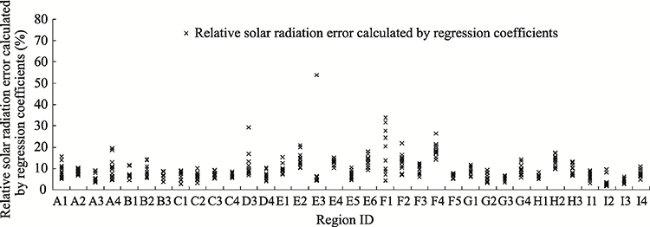
Figure 3 Relative error distribution for the Rs in each agricultural subregion calculated based on the as and bs regression coefficients
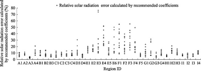
Figure 4 Relative error distribution for the Rs in each agricultural subregion calculated based on the recommended as and bs coefficients
Figure 5 shows the national mean relative Rs error calculated using the as and bs coefficients from the regression and those recommended by the FAO for every month. Based on Figure 5, we can observe that the Rs calculated using the as and bs coefficients from the re-gression is superior to the results based on the FAO recommended values for each month. The relative Rs error calculated using the former decreases by 1%-6% compared with the latter, with a large decrease in the winter and spring and a small decrease in the summer and autumn.
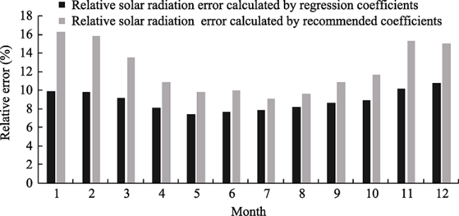
Figure 5 National monthly mean of the relative Rs errors calculated based on the regression and recommended as and bs coefficients
Figure 6 shows a comparison of the differences between the six-year mean values of the relative Rs errors calculated with the as and bs coefficients from different months in different regions and the FAO recommended values. The red lines indicate that the relative Rs error calculated via the regression results of the as and bs coefficients is less than the relative Rs error calculated via the FAO recommended values. In other words, the regression as and bs coefficients are better than the recommended coefficients. This value indicates how many months in a particular region that the regression as and bs coefficients are better than the recommended coefficients over one year. The black lines indicate the opposite of the red lines. Based on Figure 6, although the results in Figures 3 to 5 show that, overall, the Rs calculated with the as and bs coefficients based on the regression of the historical observations is better than the Rs calculated using the as and bs coefficients recommended by the FAO, for specific applications, not all Rs values calculated using the regression coefficients during all months in all of the agricultural subregions are superior to the Rs values calculated using the FAO recommended coefficients. The mean Rs error calculated using the regression coefficients was better than the Rs calculated using the FAO recommended coefficients only in Regions E, F, and I. The Rs calculated with the FAO recommended coefficients in nearly half of the entire year in Regions A, B, C, and D was better than the Rs calculated using the regression coefficients. The Rs calculated with the FAO recommended coefficients in Regions G and H for three months was better. Specifically, in the agricultural subregions, the overall trend mimicked the results for the primary regions. For example, in the agricultural subregions of Regions A, B, C, and D, there were more months when the Rs calculated using the FAO recommended coefficients was more accurate than when using the regression coefficients. In contrast, there were less months when the Rs calculated using the FAO recommended coefficients were more accurate than when using the regression coefficients in Regions E, F, and I. The other regions ranged between these two extremes. We note that there is no valid station observation data in D1 and G5. Furthermore, the results cannot be verified in the D2 region due to the absence of observation data for the verification years.
Figure 6 A comparison of the results for the relative Rs error when using the as and bs coefficient values from the regression and those recommended by the FAO: a. Region A, b. Region B, c. Region C, d. Region D, e. Region E, f. Region F, g. Region G, h. Region H, and i. Region I

4.3 Optimal coefficient determination

Based on the results of our error analysis, the regression results for the as and bs coefficients are overall more reliable than the FAO recommended coefficients. The calculated Rs error based on the regression coefficients is relatively stable throughout the year. However, the regression coefficients are not entirely reliable when used in certain agricultural subregions. Under the condition that no other methods are introduced, the simplest and most feasible scheme is to combine the application of the regression coefficients with the FAO recommended coefficients. Therefore, by comparing the Rs errors calculated using the monthly as and bs coefficients obtained via the least-squares regression and the as and bs coefficients recommended by the FAO (Figure 6), we selected the as and bs coefficients corresponding to the Rs value with the smaller errors as the final optimal values (Table 1).
Table 1 Monthly optimal values for the coefficients of the AP for each agricultural subregion in China
Region ID Jan. Feb. Mar. Apr. May. Jun. Jul. Aug. Sep. Oct. Nov. Dec.
as bs as bs as bs as bs as bs as bs as bs as bs as bs as bs as bs as bs
A1 0.36 0.32 0.20 0.62 0.32 0.48 0.18 0.62 0.25 0.50 0.25 0.50 0.25 0.50 0.25 0.50 0.25 0.50 0.19 0.62 0.21 0.62 0.36 0.29
A2 0.28 0.46 0.31 0.44 0.26 0.49 0.25 0.50 0.26 0.44 0.25 0.50 0.25 0.50 0.25 0.50 0.25 0.50 0.25 0.50 0.30 0.41 0.33 0.35
A3 0.25 0.50 0.25 0.50 0.25 0.50 0.25 0.50 0.25 0.50 0.25 0.50 0.25 0.50 0.25 0.50 0.25 0.50 0.25 0.50 0.25 0.50 0.25 0.50
A4 0.33 0.25 0.26 0.40 0.13 0.62 0.14 0.60 0.20 0.51 0.22 0.46 0.25 0.37 0.16 0.55 0.20 0.50 0.18 0.53 0.21 0.45 0.28 0.31
B1 0.47 0.24 0.43 0.32 0.37 0.39 0.29 0.46 0.25 0.50 0.25 0.50 0.25 0.50 0.25 0.50 0.27 0.50 0.26 0.53 0.37 0.38 0.45 0.25
B2 0.40 0.27 0.20 0.56 0.25 0.49 0.25 0.50 0.25 0.50 0.27 0.39 0.38 0.20 0.23 0.49 0.25 0.50 0.25 0.50 0.25 0.50 0.25 0.50
B3 0.25 0.50 0.25 0.50 0.25 0.50 0.25 0.50 0.25 0.50 0.25 0.50 0.25 0.50 0.25 0.50 0.23 0.49 0.25 0.48 0.25 0.50 0.32 0.38
C1 0.19 0.50 0.21 0.49 0.25 0.50 0.25 0.50 0.25 0.50 0.25 0.50 0.25 0.50 0.25 0.50 0.25 0.50 0.25 0.50 0.21 0.46 0.16 0.54
C2 0.23 0.46 0.25 0.50 0.31 0.37 0.13 0.66 0.26 0.43 0.22 0.48 0.25 0.50 0.25 0.39 0.27 0.37 0.20 0.52 0.19 0.54 0.22 0.47
C3 0.20 0.50 0.23 0.48 0.25 0.50 0.25 0.50 0.22 0.46 0.25 0.50 0.25 0.50 0.25 0.50 0.19 0.52 0.25 0.50 0.18 0.52 0.25 0.50
C4 0.21 0.43 0.18 0.52 0.25 0.50 0.21 0.47 0.17 0.55 0.21 0.46 0.20 0.47 0.20 0.46 0.25 0.50 0.17 0.54 0.17 0.53 0.18 0.47
D2 0.22 0.46 0.25 0.38 0.25 0.36 0.28 0.30 0.26 0.37 0.21 0.48 0.22 0.47 0.20 0.50 0.18 0.52 0.20 0.47 0.21 0.46 0.22 0.47
D3 0.24 0.44 0.25 0.50 0.25 0.50 0.18 0.55 0.15 0.60 0.14 0.61 0.18 0.55 0.18 0.54 0.15 0.59 0.13 0.62 0.19 0.52 0.17 0.54
D4 0.25 0.50 0.25 0.50 0.25 0.50 0.25 0.50 0.13 0.67 0.22 0.51 0.21 0.52 0.25 0.50 0.19 0.56 0.25 0.50 0.25 0.50 0.25 0.50
E1 0.16 0.55 0.12 0.64 0.10 0.69 0.14 0.60 0.18 0.53 0.17 0.52 0.16 0.55 0.15 0.56 0.16 0.55 0.17 0.55 0.15 0.57 0.14 0.58
E2 0.25 0.50 0.25 0.50 0.25 0.50 0.21 0.46 0.23 0.43 0.22 0.47 0.21 0.51 0.19 0.53 0.16 0.60 0.14 0.60 0.16 0.54 0.25 0.50
E3 0.10 0.73 0.11 0.70 0.11 0.67 0.12 0.63 0.17 0.55 0.17 0.55 0.18 0.53 0.15 0.59 0.11 0.71 0.19 0.53 0.16 0.58 0.16 0.56
E4 0.10 0.68 0.10 0.71 0.11 0.65 0.16 0.46 0.15 0.58 0.20 0.45 0.23 0.44 0.21 0.48 0.19 0.52 0.18 0.52 0.15 0.58 0.12 0.65
E5 0.13 0.73 0.19 0.52 0.16 0.60 0.20 0.52 0.18 0.61 0.25 0.50 0.25 0.50 0.25 0.50 0.25 0.50 0.25 0.50 0.21 0.53 0.18 0.59
E6 0.13 0.63 0.12 0.63 0.11 0.65 0.13 0.55 0.14 0.60 0.19 0.48 0.18 0.50 0.23 0.42 0.17 0.56 0.21 0.48 0.16 0.58 0.17 0.52
F1 0.16 0.59 0.19 0.51 0.18 0.55 0.35 0.17 0.26 0.40 0.20 0.54 0.24 0.48 0.19 0.59 0.15 0.68 0.18 0.56 0.24 0.37 0.22 0.48
F2 0.15 0.53 0.15 0.64 0.16 0.59 0.17 0.52 0.19 0.49 0.17 0.55 0.19 0.49 0.18 0.50 0.16 0.53 0.17 0.52 0.16 0.57 0.14 0.62
F3 0.14 0.53 0.13 0.58 0.11 0.64 0.14 0.54 0.16 0.52 0.18 0.50 0.19 0.49 0.23 0.41 0.21 0.43 0.18 0.45 0.15 0.55 0.14 0.54
F4 0.11 0.77 0.12 0.73 0.25 0.50 0.14 0.61 0.25 0.50 0.25 0.50 0.25 0.50 0.20 0.46 0.16 0.54 0.25 0.50 0.12 0.76 0.13 0.62
F5 0.20 0.56 0.25 0.50 0.13 0.63 0.19 0.53 0.20 0.52 0.22 0.48 0.23 0.46 0.21 0.51 0.22 0.51 0.25 0.50 0.18 0.59 0.16 0.61
G1 0.15 0.59 0.14 0.62 0.13 0.65 0.15 0.58 0.16 0.55 0.19 0.43 0.25 0.50 0.25 0.50 0.25 0.50 0.25 0.50 0.25 0.50 0.25 0.50
G2 0.17 0.58 0.15 0.62 0.16 0.54 0.17 0.57 0.19 0.50 0.21 0.48 0.22 0.45 0.22 0.46 0.22 0.48 0.27 0.41 0.21 0.52 0.20 0.53
G3 0.25 0.50 0.25 0.50 0.23 0.45 0.30 0.33 0.25 0.50 0.25 0.50 0.25 0.50 0.25 0.50 0.25 0.50 0.25 0.50 0.25 0.50 0.27 0.42
G4 0.19 0.54 0.25 0.50 0.25 0.50 0.25 0.50 0.25 0.50 0.25 0.50 0.34 0.28 0.25 0.50 0.28 0.34 0.25 0.50 0.25 0.50 0.21 0.50
H1 0.25 0.50 0.25 0.50 0.41 0.29 0.35 0.38 0.25 0.50 0.25 0.50 0.27 0.47 0.23 0.53 0.25 0.50 0.25 0.50 0.25 0.50 0.25 0.50
H2 0.25 0.50 0.25 0.50 0.25 0.50 0.37 0.30 0.17 0.60 0.30 0.42 0.27 0.44 0.24 0.49 0.25 0.50 0.21 0.53 0.23 0.52 0.26 0.47
H3 0.25 0.50 0.25 0.50 0.25 0.50 0.29 0.42 0.34 0.35 0.35 0.34 0.30 0.40 0.32 0.37 0.34 0.36 0.31 0.42 0.25 0.50 0.27 0.43
I1 0.16 0.73 0.34 0.49 0.39 0.39 0.25 0.50 0.40 0.36 0.43 0.32 0.35 0.45 0.35 0.45 0.38 0.39 0.25 0.50 0.25 0.50 0.25 0.50
I2 0.24 0.60 0.27 0.52 0.25 0.50 0.30 0.42 0.28 0.45 0.28 0.46 0.23 0.60 0.21 0.64 0.22 0.60 0.17 0.69 0.30 0.52 0.31 0.50
I3 0.33 0.47 0.48 0.29 0.49 0.24 0.27 0.55 0.27 0.53 0.26 0.53 0.26 0.54 0.30 0.47 0.29 0.50 0.29 0.53 0.28 0.56 0.25 0.50
I4 0.39 0.39 0.32 0.48 0.22 0.59 0.34 0.39 0.28 0.47 0.30 0.45 0.24 0.54 0.34 0.38 0.30 0.46 0.43 0.35 0.22 0.61 0.23 0.60

Note: Due to the absence of valid observation station data in D1 and G5, the coefficient correction results are missing. Stations in D2 have no valid observation data from 2011 to 2016, such that we have not verified the results for D2.

5 Discussion

The factors that affect Rs mainly include the latitude, season, altitude, slope direction (shelter), climate, and weather. Among these factors, the latitude and seasonal changes determine the position of direct sunlight on the surface and the maximum sunshine duration. Under specific spatio-temporal conditions, these two variables can be regarded as fixed values, thus determining the initial value of the solar radiation that reaches the surface. Under the assumption that the surface morphology is uniform and there is no atmosphere, the initial value is Ra. However, owing to the uneven surface morphology and existence of the atmosphere, the solar radiation that reaches the surface has spatio-temporal changes, leading to the changes in the as and bs coefficients in different agricultural regions.
The shape and gravitation characteristics of the Earth objectively produce regional differences in the surface atmospheric composition and thickness, which first reflects the defects of the fixed as and bs coefficients. In addition, the composition and thickness of the atmosphere also change under the influence of the climate, changes in the seasons, and human activity. However, in the existing regression correction schemes for the as and bs coefficients (Peng et al., 2006; Yin et al., 2008; Liu et al., 2009a; Liu et al., 2009b; Hu et al., 2010; Liu et al., 2010; Li et al., 2012a; Li et al., 2012b; Cao et al., 2014; Paulescu et al., 2016; Yuan et al., 2018; Huang et al., 2019; Xia et al., 2020a; Xia et al., 2020b), fixed as and bs coefficients are mostly obtained based on the time scale of the acquired data, rather than dynamic as and bs coefficients that change with time. Therefore, we conducted a regression analysis of multi-year data month by month, obtaining the as and bs values in different agricultural regions month by month to reflect the seasonal changes in the as and bs coefficients in different agricultural regions throughout a year. Compared with the correction results for the as and bs coefficients of various agricultural regions in China based on an annual scale reported in Xia et al. (2020b), we observe that the root mean square error (RMSE) and mean relative error (MRE) of the Rs calculated using the as and bs coefficients from the monthly regressions are superior to the as and bs coefficients fixed within the year (Figure 7). The Nash-Sutcliffe efficiency coefficient (NSE) results corresponding to the monthly coefficients are larger than the NSE results corresponding to the fixed coefficients (Figure 7). This indicates that seasonal changes in China have a certain influence on the values of the as and bs coefficients. For accurate estimation of Rs, we cannot ignore the fact that the as and bs coefficients change with the seasons.
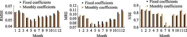
Figure 7 A comparison of the mean monthly values of the RMSE, MRE, and NSE from 2011 to 2016 between the fixed as and bs coefficients, regressed at an annual scale, and the monthly regressed as and bs coefficients
Xia et al.’s study (2019) is the only one that discusses the influence that the length change in the observed time series has on the as and bs coefficients based on the obtained fixed as and bs coefficients within a year. We are not aware of any other relevant study. In this study, we selected Subregion C3, which is characterized by relatively flat terrain. Discontinuities in the station data were avoided by taking the average value of the valid observation data from stations in the region. Using five years as the starting point and a step size of the data volume, we obtained the as and bs coefficients under different data series lengths of four months via regression (Figure 8). Based on Figure 8, we observe that the as coefficient essentially remains unchanged in the winter (January). In the spring (April), its value decreases with an increase in the data series length. In summer (July), the coefficient values for a data series length of five years is the smallest, the values remain essentially unchanged for a data series length of 10 to 40 years, and there is a sudden increase in the values for a data series length of 45 to 50 years. In autumn (October), the values fluctuate, but the range is not large. The bs coefficient is characterized by stable fluctuations in autumn and winter. The spring exhibits a trend of increased volatility while in summer there is a decrease in the fluctuations. Thus, we can observe that the time series length of the observed data has more or less of an influence on the as and bs coefficients. In other words, the sensitivity of the as and bs coefficients to the length of the regression data series varies in different months, which has not been taken into account in existing studies, including this study. In addition, by observing the change in the average estimated Rs relative error for the application from 2011 to 2015 of the as and bs coefficients for the monthly regression of different time-series data (Figure 9), we observe that the average estimated Rs error corresponds to the 10-year time series data, which is generally lower than that of the other time series. This indicates that the regression of the as and bs coefficients has an optimal data series length, where the influence of the estimated Rs accuracy may be sensitive to a change in the data series length of less than 15 years. The influence of the Rs accuracy may not be sensitive to a change in the data series length of more than 15 years. Therefore, we must discuss the inter-annual changes in the as and bs coefficients month by month across the country in future studies.
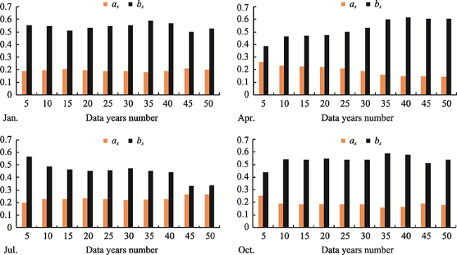
Figure 8 The as and bs coefficients for the monthly regression in region C3 with varying lengths of the time series data
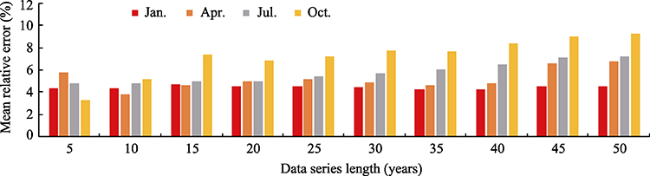
Figure 9 The mean relative errors for the as and bs coefficients regressed monthly by different time series data in region C3 from 2011 to 2015
The existing regression correction schemes for the as and bs coefficients may also smooth out the random weather changes in different seasons and the changes in the atmospheric characteristics caused by the discharge of large amounts of pollutants into the atmosphere by human activity within a short period in local regions. Higher altitudes have shorter solar radiation transmission paths and elevated as and bs coefficients. A sunny slope can receive direct solar energy, such that the as and bs coefficients of a sunny slope are greater than those of a shaded slope. In existing studies and here, coefficient correction of the AP is based on observation data from meteorological stations, which are typically located on open, sunny ground. Therefore, the influence that the slope orientation (shielding objects) has on the as and bs coefficients is not considered under the existing data observation conditions. This study mainly aims to lend support for the calculation of ET0. Therefore, the average values of the as and bs coefficients at the regional stations were obtained based on China’s Comprehensive Agricultural Regionalization. However, this division does not actually correspond to the above factors that affect the spatial and temporal characteristics of surface solar radiation, such that a value for the entire region based on the average results of the stations within the agricultural divisions also leads to errors. For example, in studies based on independent stations, altitude is also a fixed value, which does not need to be considered. However, regionalization studies of these coefficients predominantly use the average value of a region (Hu et al., 2010; Huang et al., 2019), which is equivalent to the value based on the average regional altitude. This study is no exception, where the average values of as and bs were used to represent the values of the entire agricultural region based on the regional statistics of the comprehensive agricultural regionalization. In Figure 1, we observe that the spatial distribution of meteorological stations in China is relatively dense in the southeast and sparse in the northwest, such that the density of stations in each agricultural subregion is different. The average value in each subregion may be different with respect to the accuracy due to differences in sample size. Therefore, if these are used to support other research or applications, such as solar energy engineering research and applications, they would require further analysis of the correlations between the station as and bs coefficients and certain elements, such as topography, to improve the spatial scalability of the as and bs coefficients and the realization of grid as and bs coefficients to extend their application fields.

6 Conclusions

Using the least-squares regression method, this study, based on meteorological observation data from 121 stations in China, calculated the coefficients of the AP month by month in 36 agricultural subregions of China. By comparing the Rs errors estimated using the values of the as and bs coefficients obtained by a monthly regression and the values of the as and bs coefficients suggested by the FAO, we selected the values of the as and bs coefficients corresponding to the Rs values with the smallest estimation errors as the final applied values of the coefficients for the AP. The main conclusions of our study are as follows.
(1) The values of the coefficients for the AP calculated in this study showed no uniform variation trends with respect to the spatial and temporal distribution of the nine agricultural regions, which is consistent with the spatio-temporal difference characteristics of the unstable atmospheric environment. Moreover, the regression values in most agricultural subregions were different from the global fixed values recommended by the FAO (as = 0.25, bs = 0.50). Therefore, we must discuss the differences in the accuracy between the localized values of the coefficients for the AP and the global fixed values to optimize the applied values of the as and bs coefficients.
(2) Overall, the relative accuracy of the Rs calculated using the regression as and bs coefficients is better than that calculated using the values recommended by the FAO. However, for specific applications in each agricultural region, the Rs accuracy based on the as and bs coefficients from the two sources is not equal. Therefore, by integrating the different scales of the Rs estimation accuracy, from an entire application perspective, we suggest that Regions A, B, C, D, and H continue to use the as and bs coefficients recommended by the FAO for the AP, whereas the other four regions (E, F, G and I) should adopt the as and bs coefficients based on the least-squares regression presented in this study. In specific agricultural subregions with higher accuracy requirements or smaller-scale applications, we recommend the use of the optimized coefficients for the monthly calculation of Rs.
This study enriches the overall investigation of the AP coefficient correction and has certain reference value for improving the calculation of ET0. Although we provide the AP coefficients supporting ET0 calculations in each agricultural region based on existing data conditions and by monthly regression, verification, and optimization, there are still some deficiencies that require further exploration. 1) This study only discussed the localization of the as and bs coefficients based on monthly scale data. A more sophisticated ten-day scale or daily coefficients may be more pertinent in the fields of Earth science and solar energy engineering, such that we must collect finer time scale data for in-depth research. 2) Discussing the influence that the length of the time series data has on the monthly as and bs coefficients is necessary. Based on the determination of the optimal historical data series length, the factors that affect the as and bs coefficients can be further analyzed to improve the accuracy of the applied values of the as and bs coefficients. 3) The as and bs coefficients themselves are reflections of the solar radiation atmospheric transmittance, where, at its present stage, remote sensing technology has achieved fruitful results in the inversion of atmospheric indicators. Moreover, based on the principle of energy balance, previous studies have proposed numerous expressions for solar radiation atmospheric transmittance. Therefore, to explore the relationship between the as and bs coefficients and atmospheric parameters obtained via remote sensing inversion (such as the aerosol optical thickness or density), as well as based on the existing expression of the atmospheric transmissibility of solar radiation, building values for grid as and bs coefficients are also a potential breakthrough for the refined application of the AP.
[1]
Akinoğlu B G, Ecevit A, 1990. A further comparison and discussion of sunshine-based models to estimate global solar radiation. Energy, 15:865-872.

DOI

[2]
Allen R G, Pereira L S, Raes D et al., 1998. Crop evapotranspiration: Guidelines for computing crop water requirements. FAO irrigation and drainage Paper 56. FAO, Rome, 300(9):D05109.

[3]
Almorox J, Hontoria C, 2004. Global solar radiation estimation using sunshine duration in Spain. Energy Conversion and Management, 45:1529-1535.

DOI

[4]
Ångström A, 1924. Solar and terrestrial radiation. Report to the international commission for solar research on actinometric investigations of solar and atmospheric radiation. Quarterly Journal of the Royal Meteorological Society, 50:121-126.

DOI

[5]
Cao W, Xu Y, Duan C, 2014. Research on applicability of solar radiation parametric model in Anhui Province. Chinese Agricultural Science Bulletin, 30:207-212. (in Chinese)

[6]
Chen J, Liu H, Wu W et al., 2011. Estimation of monthly solar radiation from measured temperatures using support vector machines: A case study. Renewable Energy, 36:413-420.

DOI

[7]
Cui R, 2014. The analysis of spatiotemporal variation characteristics of global solar radiation in Shandong Province. Journal of Natural Resources, 29:1780-1791. (in Chinese)

[8]
Du Y, Mao H, Liu A et al., 2003. The Climatological calculation and distributive character of global solar radiation in Guangdong Province. Resources Science, 25:66-70. (in Chinese)

[9]
Ertekin C, Yaldiz O, 2000. Comparison of some existing models for estimating global solar radiation for Antalya (Turkey). Energy Conversion and Management, 41:311-330.

DOI

[10]
Glover J, McCulloch J S G, 1958. The empirical relation between solar radiation and hours of sunshine. Quarterly Journal of the Royal Meteorological Society, 84:172-175.

DOI

[11]
Gopinathan K K, 1988. A general formula for computing the coefficients of the correlation connecting global solar radiation to sunshine duration. Solar Energy, 41:499-502.

DOI

[12]
Halouani N, Nguyen C T, Vo-Ngoc D, 1993. Calculation of monthly average global solar radiation on horizontal surfaces using daily hours of bright sunshine. Solar Energy, 50:247-258.

DOI

[13]
Hu Q, Yang D, Wang Y et al., 2010. Effects of Ångström coefficients on ET0 estimation and the applicability of FAO recommended coefficient values in China. Advances in Water Science, 21:644-652. (in Chinese)

[14]
Huang Z, Guo Y, Zhang Y et al., 2019. Using the Ångström-Prescott formula to calculate solar radiation from sunshine duration in China. Journal of Irrigation and Drainage, 38:77-83. (in Chinese)

[15]
Iziomon M G, Mayer H, 2002. Assessment of some global solar radiation parameterizations. Journal of Atmospheric and Solar-Terrestrial Physics, 64:1631-1643.

DOI

[16]
Ju X, Tu Q, Li Q et al., 2005. Discussion on the climatological calculation of solar radiation. Journal of Nanjing Institute of Meteorology, 28:516-521. (in Chinese)

[17]
Li M, Fan L, Liu H et al., 2012a. Impact of time interval on the Ångström-Prescott coefficients and their interchangeability in estimating radiation. Renewable Energy, 44:431-438.

DOI

[18]
Li M, Liu H, Guo P et al., 2010. Estimation of daily solar radiation from routinely observed meteorological data in Chongqing, China. Energy Conversion and Management, 51:2575-2579.

DOI

[19]
Li M, Mei X, Zhong X et al., 2012b. Parameterization of Ångström-Prescott radiation model in Yunnan Province. Transactions of the Chinese Society of Agricultural Engineering, 28:100-105. (in Chinese)

[20]
Liu J, Pan T, Chen D et al., 2017. An improved Ångström-type model for estimating solar radiation over the Tibetan Plateau. Energies, 10:892.

DOI

[21]
Liu X, Li Y, Zhong X et al., 2014. Towards increasing availability of the Ångström-Prescott radiation parameters across China: Spatial trend and modeling. Energy Conversion and Management, 87:975-989.

DOI

[22]
Liu X, Mei X, Li Y et al., 2009a. Variation in reference crop evapotranspiration caused by the Ångström-Prescott coefficient: Locally calibrated versus the FAO recommended. Agricultural Water Management, 96:1137-1145.

DOI

[23]
Liu X, Mei X, Li Y et al., 2009b. Calibration of the Ångström-Prescott coefficients (a, b) under different time scales and their impacts in estimating global solar radiation in the Yellow River Basin. Agricultural and Forest Meteorology, 149:697-710.

DOI

[24]
Liu X, Mei X, Li Y et al., 2010. Choice of the Ångström-Prescott coefficients: Are time-dependent ones better than fixed ones in modeling global solar irradiance? Energy Conversion and Management, 51:2565-2574.

DOI

[25]
Liu Y, Tan Q, Pan T, 2019. Determining the parameters of the Ångström-Prescott model for estimating solar radiation in different regions of China: Calibration and modeling. Earth and Space Science, 6:1976-1986.

DOI

[26]
Lu Y, Tian H, Lu J et al., 2016. Spatial-temporal variation characteristics of gross solar radiation in Anhui Province from 1961 to 2010. Meteorological Science & Technology, 44:769-775. (in Chinese)

[27]
Ma J, Luo Y, Shen Y et al., 2013. Regional long-term trend of ground solar radiation in China over the past 50 years. Science China Earth Sciences, 56:1242-1253.

DOI

[28]
Mai Miao, Huo Y, Zeng Y et al., 2012. The distribution characteristics of total solar radiation in Jiangsu Province. Journal of the Meteorological Sciences, 32:269-274. (in Chinese)

[29]
Ododo J C, Sulaiman A T, Aidan J et al., 1995. The importance of maximum air temperature in the parameterisation of solar radiation in Nigeria. Renewable Energy, 6:751-763.

DOI

[30]
Ögelman H, Ecevit A, Tasdemiroǧlu E, 1984. A new method for estimating solar radiation from bright sunshine data. Solar Energy, 33:619-625.

DOI

[31]
Ojosu J O, Komolafe L K, 1987. Models for estimating solar radiation availability in south western Nigeria. Nigerian Journal of Solar Energy, 6:69-77.

[32]
Olseth J A, Skartveit A, 2001. Solar irradiance, sunshine duration and daylight illuminance derived from METEOSAT data for some European sites. Theoretical and Applied Climatology, 69:239-252.

DOI

[33]
Pan T, Wu S, Dai E et al., 2013. Estimating the daily global solar radiation spatial distribution from diurnal temperature ranges over the Tibetan Plateau in China. Applied Energy, 107:384-393.

DOI

[34]
Paulescu M, Paulescu E, Gravila P et al., 2013. Weather modeling and forecasting of PV systems operation. Springer, London.

[35]
Paulescu M, Stefu N, Calinoiu D et al., 2016. Ångström-Prescott equation: Physical basis, empirical models and sensitivity analysis. Renewable and Sustainable Energy Reviews, 62:495-506.

DOI

[36]
Peng S, Xu J, Ding J et al., 2006. Influence of as and bs values on determination of reference crop evapotranspiration by Penman-Monteith formula. Journal of Irrigation and Drainage, 25:5-8. (in Chinese)

[37]
Prescott J A, 1940. Evaporation from a water surface in relation to solar radiation. Transactions of the Royal Society of South Australia, 64:114-122.

[38]
Qin J, Chen Z, Yang K et al., 2011. Estimation of monthly-mean daily global solar radiation based on MODIS and TRMM products. Applied Energy, 88:2480-2489.

DOI

[39]
Richardson C W, 1981. Stochastic simulation of daily precipitation, temperature, and solar radiation. Water Resources Research, 17:182-190.

DOI

[40]
Trnka M, Žalud Z, Eitzinger J et al., 2005. Global solar radiation in central European lowlands estimated by various empirical formulae. Agricultural and Forest Meteorology, 131:54-76.

DOI

[41]
Wen D, 1964. Discussion on the climatological calculation of solar radiation. Acta Meteorologica Sinica, 3:54-65. (in Chinese)

[42]
Xia X, Zhu X, Pan Y et al., 2019. Calibration and optimization of the Ångström-Prescott coefficients for calculating ET0 within a year in China: The best corrected data time scale and optimization parameters. Water, 11:1706.

DOI

[43]
Xia X, Zhu X, Pan Y et al., 2020a. Influence of solar radiation empirical values on reference crop evapotranspiration calculation in different regions of China. Transactions of the Chinese Society for Agricultural Machinery, 51:254-266. (in Chinese)

[44]
Xia X, Zhu X, Pan Y et al., 2020b. Parameter calibration and optimization of Ångström equation in mainland of China within a yearly scale. Journal of Irrigation and Drainage, 39:122-129. (in Chinese)

[45]
Yang G, Wang Z, Wang H et al., 2009. Potential evapotranspiration evolution rule and its sensitivity analysis in Haihe River Basin. Advances in Water Science, 20:409-415. (in Chinese)

[46]
Yin Y, Wu S, Zheng D et al., 2008. Radiation calibration of FAO 56 Penman-Monteith model to estimate reference crop evapotranspiration in China. Agricultural Water Management, 95:77-84.

DOI

[47]
Yorukoglu M, Celik A N, 2006. A critical review on the estimation of daily global solar radiation from sunshine duration. Energy Conversion and Management, 47:2441-2450.

DOI

[48]
Yuan H, Yuan X, Tang G et al., 2018. Correction of parameters in Ångström formula and analysis of total solar radiation characteristics in Huaibei plain. Journal of Drainage and Irrigation Machinery Engineering, 36:64-70. (in Chinese)

[49]
Zhang Q, Cui N, Feng Y et al., 2018. Comparative analysis of global solar radiation models in different regions of China. Advances in Meteorology, 3894831.

[50]
Zhao J, Li W, Li F, 2008. Climatological calculation and analysis of global solar radiation in the Loess Plateau. Arid Zone Research, 25:53-58. (in Chinese)

DOI

[51]
Zhou J, Wu Y, Gang Y, 2005. General formula for estimation of monthly average daily global solar radiation in China. Energy Conversion and Management, 46:257-268.

DOI

Outlines

/