Research Articles

Neighborhood impacts on household participation in payments for ecosystem services programs in a Chinese nature reserve: A methodological exploration

  • ZHANG Huijie , 1, 2, 3 ,
  • AN Li 1, 3 ,
  • BILSBORROW Richard 4 ,
  • CHUN Yongwan 5 ,
  • YANG Shuang 1, 2 ,
  • DAI Jie 1, 2, 3
Expand
  • 1. Department of Geography, San Diego State University, San Diego, CA, USA
  • 2. Department of Geography, University of California, Santa Barbara, CA, USA
  • 3. Center for Complex Human-Environment Systems, San Diego State University, San Diego, CA, USA
  • 4. Departments of Biostatistics and Geography and Carolina Population Center, University of North Carolina at Chapel Hill, USA
  • 5. School of Economic, Political and Policy Sciences, University of Texas at Dallas, Richardson, TX, USA

Zhang Huijie, PhD Student, specialized in remote sensing image processing and analysis, and spatial data analysis. E-mail:

Received date: 2020-08-13

  Accepted date: 2021-02-09

  Online published: 2021-08-25

Supported by

National Science Foundation under the Dynamics of Coupled Natural and Human Systems Program(DEB-1212183)

National Science Foundation under the Dynamics of Coupled Natural and Human Systems Program(BCS-1826839)

PES program duration for three different scenarios

Population Research Infrastructure Program(P2C)

Population Research Infrastructure Program(HD050924)

Abstract

Payments for Ecosystem Services (PES) programs have been implemented in both developing and developed countries to conserve ecosystems and the vital services they provide. These programs also often seek to maintain or improve the economic wellbeing of the populations living in the corresponding (usually rural) areas. Previous studies suggest that PES policy design, presence or absence of concurrent PES programs, and a variety of socioeconomic and demographic factors can influence decisions of households to participate or not in the PES program. However, neighborhood impacts on household participation in PES have rarely been addressed. This study explores potential neighborhood effects on villagers’ enrollment in the Grain-to-Green Program (GTGP), one of the largest PES programs in the world, using data from China’s Fanjingshan National Nature Reserve. We utilize a fixed effects logistic regression model in combination with the eigenvector spatial filtering (ESF) method to explore whether neighborhood size affects household enrollment in GTGP. By comparing the results with and without ESF, we find that the ESF method can help account for spatial autocorrelation properly and reveal neighborhood impacts that are otherwise hidden, including the effects of area of forest enrolled in a concurrent PES program, gender and household size. The method can thus uncover mechanisms previously undetected due to not taking into account neighborhood impacts and thus provides an additional way to account for neighborhood impacts in PES programs and other studies.

Cite this article

ZHANG Huijie , AN Li , BILSBORROW Richard , CHUN Yongwan , YANG Shuang , DAI Jie . Neighborhood impacts on household participation in payments for ecosystem services programs in a Chinese nature reserve: A methodological exploration[J]. Journal of Geographical Sciences, 2021 , 31(6) : 899 -922 . DOI: 10.1007/s11442-021-1877-1

1 Introduction

Recent years have witnessed a number of studies of neighborhood impacts on human decision-making. The concept of “neighborhood” (similar to community), via its effects on people’s attitudes and values, has been found to be fundamental in many fields, including human ecology, sociology, and demography. Neighborhoods/communities in which people live influence attitudes and activities because people living in the same geographic area possess the same or similar natural and social environments and interact with each other (Lee et al., 1994). Individuals learn from neighbors, make adjustments, and make decisions (Foster and Rosenzweig, 1995). As a result, social norms are formed within neighborhoods of various sizes, in which people follow these norms (Coleman, 1994; Bendor and Swistak, 2001; White and Johnson, 2016). However, the appropriate definition of neighborhood has been found to vary depending on the specific context, including the topic of study, data available, and scientific method(s) used. In general, neighborhood impacts come into play due to social interactions, affecting social norms and individual behavior (Dietz, 2002). The term neighborhood impact has also been used in spatial data analysis involving distance decay to address spatial autocorrelation (Case, 1992; Page and Solon, 2003).
The importance of this concept dates back to the classic sociological study of Amos Hawley (1950): “From a spatial standpoint, the community may be defined as comprising that area the resident population of which is interrelated and integrated with reference to its daily requirements”. Residents within the same neighborhood often affect (and are affected by) each other’s values, attitudes, decisions, and activities, making data about these individuals correlated. If we use such correlated data directly without considering neighborhood effects, there is a high chance of generating biased modeling results and misinterpreting people’s decisions or behavior (Bilsborrow et al., 1984; Chen et al., 2009; Zvoleff et al., 2013; Bilsborrow 2016; Sullivan et al., 2017).
One domain to examine potential neighborhood effects on human decision-making is to evaluate people’s participation in payments for ecosystem services (PES) programs, for several reasons. First, ecosystem preservation and restoration is naturally challenging: an ecosystem is embedded in geographic space, with processes and functions operating at varying spatial scales. Such processes and functions, if intervened by major disturbances (e.g., natural disasters, human actions), may dysfunction or even fail. This fact may explain—at least partially—some unsuccessful reports of PES implementation over the last 2-3 decades (Pattanayaket al., 2010). Second, PES programs offer incentives to landowners so that they change land use decisions to maintain or restore ecosystem services (Jack et al., 2008; Wunder, 2005, 2008). The PES programs require voluntary participation of landowners (Wunder, 2005), so factors that influence landowners’ participation and compliance are likely to affect the effectiveness of the PES program (Kaczanet al., 2013; Bremer et al., 2014). Previous PES studies have found that a variety of factors, such as program implementation procedures, local social norms, and the existence of concurrent PES programs, may affect household enrollment decisions (Chen et al., 2009; Layton and Siikamäki, 2009; Nordén, 2014; Sarkissian et al., 2017; Sorice et al., 2018; Yost et al., 2020).
Nevertheless, there is little empirical evidence regarding whether or how spatial factors, defined as neighborhoods of various sizes, may affect household participation in PES programs. Households within a neighborhood may share characteristics due to spatial autocorrelation in seemingly “non-spatial” ways (Sullivan et al., 2017). Therefore, it is important to account for neighborhood impacts, if any, when seeking to understand household enrollment decisions in PES.
In this context, we examine the Grain-to-Green Program (GTGP) in Fanjingshan National Nature Reserve (FNNR), Guizhou Province, China. The GTGP, one of the largest PES programs in the world, aims to persuade farmers to convert cropland on sloping land back to forest or grassland (Liu et al., 2008; Chen et al., 2009). The purpose of this study is to explore whether and how much neighborhood effects affect household participation in GTGP in the FNNR. The eigenvector spatial filtering (ESF) technique (Griffith et al., 2019), integrated with fixed effects logistic regression models (FELRM), is employed to study how non-spatial factors, after accounting for neighborhood impacts, impact household enrollment in GTGP. This paper extends the work of Yost et al. (2020), which explored the influences of non-spatial factors on farmers’ participation in GTGP in the FNNR. In this study, we test whether and how household decisions to enroll or not are affected by neighborhood effects, controlling for socioeconomic and demographic factors.

2 Background

2.1 The Grain-to-Green Program

The Grain-to-Green Program (GTGP), one of the largest ecological restoration programs in the world, has been implemented in China starting in 1999 (Feng et al., 2013). The Chinese government has spent about 28.8 billion USD on GTGP during the 1999-2008 period (Lüet al., 2012), with a commitment to invest a total of more than 40 billion USD by 2050 (Feng et al., 2013, 2016). The goal of GTGP is to significantly reduce soil erosion and land desertification by converting cultivated land to forest or grassland (Uchid et al., 2009). The main criterion for enrolling land in GTGP is that the slope of the farmland must be greater than 25° in southwestern China and greater than 15° in northwestern China (Chenet al., 2009). By 2008, 9.27 million ha of farmlands had been transferred to forestland or grassland through GTGP (Liu et al., 2008). There are some alternative names of GTGP which aims at increasing forestland and reducing farmland, such as Sloping Land Conversion Program (SLCP) (Lu and Yin, 2020), Conversion of Cropland to Forest Program (CCFP) (Wang et al., 2020; Zhang et al., 2020), and Returning Farmland to Forest Program (RFFP) (Li et al., 2019; Li et al., 2020).
The ecological effects of GTGP were already noticeable nationwide in that vegetation coverage increased, water surface runoff declined, and soil erosion was effectively controlled (Long et al., 2006; Xu et al., 2006; Wang et al., 2016) as the forest area grew by 952,000 ha from 2000 to 2005 (Yang, 2006). In addition, there were positive socioeconomic impacts of GTGP, including poverty alleviation and substantial changes in household income structures due to shifting from on-farm work to off-farm work (Liu et al., 2008). Regardless of these reported benefits, there still exists considerable uncertainty regarding GTGP design and implementation, perhaps precluding maximum household participation (Adhikari and Boag, 2013).
Previous studies revealed that household enrollment in PES programs is influenced by PES program features (Zbinden and Lee, 2005; Adhikari and Boag, 2013; Adhikari and Agrawal, 2014; Nordén, 2014; Zhang et al., 2018a), social norms (Chen et al., 2012, 2009), whether there are concurrent PES programs (Yost et al., 2020), and socioeconomic and demographic factors (Layton and Siikamäki, 2009; Kaczan et al., 2013; Bremer et al., 2014; Chen et al., 2017). The amount of payment is one of the major factors, yet not the only one, that affects household enrollment in PES programs (Sarkissian et al., 2017; Sorice et al., 2018). Other factors include program duration, land use options for enrolled parcels, social norms in the local community, presence of concurrent PES programs, gender of household head, education, financial capital, and household economic factors (Zbinden and Lee, 2005; Chen et al., 2009, 2012; Gillenwater, 2012; Balderas et al., 2013; Bremer et al., 2014; Chen et al., 2017; Zhang et al., 2018b; Yost et al., 2020). In the existing literature regarding PES participation, however, little is known about the role of neighborhood impacts.
Guizhou Province is located in southwest China. About 73% of the area has developed karst landforms and suffers varying levels of soil erosion because of excessive logging and conversion to farmland on its steep slopes (Xu et al., 2008; Zhang et al., 2007). FNNR in Guizhou Province was one of the first regions to participate in the GTGP, starting in 2000 when 774 households participated with a total of 1296 mu (1 mu = 1/15 ha). Local farmers received an average of 230 yuan/mu/year from 2000, but the compensation dropped to 134 yuan/mu/year starting in 2007. The GTGP policy always allowed farmers to plant ecological trees such as Chinese fir (Cunninghamia lanceolata), but sometimes did and sometimes did not allow planting economic or commercial trees such as tea (Camellia sinensis) which provided cash incomes after only a few years. Usually the local government provided seedlings to participating households for planting on the enrolled land parcels. By enrolling farmland in GTGP, participants were freed up from on-farm work on that land and thus expected to be more likely to seek off-farm employment, giving rise to increases in overall household income and less reliance on agriculture (Liu and Diamond, 2005; Uchida et al., 2009).

2.2 Neighborhood impacts

Neighborhood effects on human decision-making are likely affecting local people’s GTGP enrolment decisions, yet little is known about such effects. As an example, Murray and Gottsegen (1997) employed a location planning model, where block groups were aggregated to different sizes for location planning in the Buffalo (US) metropolitan area. They found that different degrees of aggregation led to the same optimal solution with high stability. On the other hand, Sullivan et al. (2017) found neighborhood size was influential in affecting collective actions to remove the invasive species, Mikania micrantha, that had degraded local socio-ecological systems and human wellbeing. Also, neighbor’s opinions were found to influence household decisions about removing invasive species after other relevant factors were controlled (Sullivanet al., 2017).
Nevertheless, the literature on household enrollment in PES programs has focused on PES program aspects and the impact of socioeconomic, demographic, geographic, and environmental factors, ignoring interactions among people and households. Not considering neighborhood factors (expressed statistically as spatial autocorrelation) is likely to lead to biased regression coefficients of the factors studied (An et al., 2016; Sullivan et al., 2017). Furthermore, it is especially important to account for neighborhood impacts from a policy perspective, as policy-makers and implementers seek to maximize the collaboration of neighboring landholders to achieve the intended conservation goals (e.g., reforestation).

2.3 Eigenvector spatial filtering

The eigenvector spatial filtering (ESF) method is a relatively recent, non-parametric statistical approach for dealing with spatial autocorrelation (Griffith, 2000; Chun, 2008). Compared with the spatial autoregressive (SAR) model, the ESF method provides a more flexible way to account for spatial autocorrelation impacts as the SAR approach uses the maximum likelihood method for parameter estimation, which becomes unreliable for small datasets (Burden et al., 2015). In addition, the ESF method can be utilized for non-Gaussian models, including logistic regression and Poisson regression (Griffith et al., 2019). The aim of the ESF method is to decompose key variables in multiple regression models into spatial and non-spatial components. Given locational information (often x,y coordinates) of all records or observations in a dataset, the ESF method extracts a set of eigenvectors from a given contiguity matrix, which is defined as:
$MCM=\left( I-\frac{{{11}^{T}}}{n} \right)C\left( I-\frac{{{11}^{T}}}{n} \right)$,
where Iis an n × nidentity matrix, 1 indicates an n×1 matrix or a column vector withn rows of 1; Trepresents the operation of transposing a matrix, Cis an n× nbinary spatial weights matrix; and n is the number of observations. It is noted that the eigenvectors E1, E2, …, En are orthogonal and associated with the corresponding eigenvalues λ1>λ2>...>λn (Chun and Griffith, 2013). Eigenvectors can be selected to enter the regression model to eliminate spatial autocorrelation (Tiefelsdorf and Griffith, 2007; Griffith, 2000; Chun and Griffith, 2011). A useful way to select the most influential eigenvectors is a stepwise procedure (Chun et al., 2016), but it is slow when the number of observations is large. The least absolute shrinkage and selection operator (LASSO) has thus been proposed to increase efficiency, and is much faster than the stepwise procedure (Seya et al., 2015). In addition, some studies have revealed that it is also a practical way to choose the top keigenvectors to account for neighborhood impacts with extensive research devoted to determining k (Chun and Griffith, 2011; An et al., 2016; Sullivan et al., 2017).
The ESF method has been used in recent years in studying migration (Clairfontaine et al., 2015; Griffith et al., 2017; Liu and Shen, 2017), real estate prices (Clairfontaine et al., 2015; Griffith et al., 2017; Liu and Shen, 2017), crime distribution and dynamics (Chun, 2014; Helbich and Arsanjani, 2015; Medina et al., 2018), and ecological and biogeographical issues (Michel and Knouft, 2014; Sternberg et al., 2014; Yang et al., 2014; Lara et al., 2016). As people residing in the same or close neighorhoods tend to be similar in a variety of dimensions, e.g., values, attitudes, incomes, physical environments, and policy contexts, this leads to spatial autocorrelation in those measures. The conceptual link between neighborhood effects and spatial autocorrelation thus makes methods dealing with the latter good candidates to handle neighborhood effects. However, there are few studies on how neighborhood features, through the construction of spatial units (i.e., aggregating data records) affect regression results. The ESF method thus has important potential to partition the values of certain variables into a component due to neighborhood effects (spatial autocorrelation) and a component independent of neighborhood effects. To the best of our knowledge, no previous study has used the ESF method to do this for evaluating the effects of conventional factors on household participation in PES programs, as proposed here. Specifically, we will explore the effects of defining neighborhoods of varying size to correct for the usual regression bias, recovering the hidden (due to neighborhood effects) “role” of relevant variables.

3 Methods

3.1 Study site and data collection

This study aims to identify the unbiased effects of variables on household enrollment decisions (in GTGP) after correcting potential neighborhood-induced confounding impacts in a key ecological study area in China. The study site is Fanjingshan National Nature Reserve (27º44´42˝-28º03´11˝N, 108º34´19˝-108º48´30˝E) located in the Wuling Mountains, Guizhou Province, Southwest China (Figure 1). FNNR is a UNESCO Biosphere Reserve (I.W.H.E. Report), which has a humid and mid-subtropical monsoon climate with hot and humid summers and mild winters. FNNR provides habitats for many wildlife species designated as endangered by the Chinese government, such as the Guizhou snub-nosed monkey (Rhinopithecus brelichi), the Asiatic black bear (Ursus thibetanus), and Elliot’s pheasant (Syrmaticus ellioti) (Yang et al., 2002). Moreover, FNNR is home to several endangered plant species, including the dove-tree (Davidia involucrata) and the Fangjinshan fir (Abiesfanjingshanensis) (GEF Project Team, 2004). The steep terrain also helps provide habitats for various other species, but increases the risk of soil erosion.
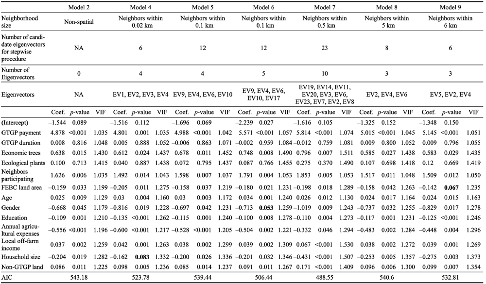
Figure 1 Fanjingshan National Reserve and sample households in the study site. The core zone designation was based on both conservation goals and local people’s livelihood needs, resulting in a small number of households located within the core zone. At the same time, some households were included in the survey and subsequent data analysis even though they are just outside the reserve’s boundary because they affect the reserve through various activities such as fuelwood collection and collection of medicinal herbs.
There are about 13,000 indigenous people living in the 3256 households inside and in the immediate buffer zone of FNNR (An et al., 2020). In order to conduct a household survey in 2014, a representative probability sample of 605 households was selected for interview using a stratified random sampling strategy (for sampling and survey details, see Yost et al., 2020). One adult from each household was selected to respond, most often the household head. Out of the 605 households, a subset of about one quarter was selected for carrying out 435 experiments (three per household: see Yost et al., 2020 for experiment details). The resulting 147 households have x and y geographic coordinates and complete data for other variables used in the data analysis.
Payment levels, program duration, and whether neighbors are perceived to be willing to participate are considered a priori potentially important variables affecting individual household decisions to participate in PES programs (Chen et al., 2009; Tsitrou et al., 2013; Bremer et al., 2014; Sorice et al., 2018). Following a pretest based on 29 households, Yost et al. (2020) developed three hypothetical scenarios for each of four program components: PES payment level, PES program duration, post-enrollment land use options allowed, and perceived participation levels of neighbors. Each of these four hypothetical variables was allowed to have three values, from which the interviewer randomly chose one, combined to form a policy scenario. Under a given scenario, we then asked the household respondent if he/she would be willing to enroll farmland (additional, if already had enrolled some) in the Grain-to-Green Program (GTGP). Data collected on the respondent’s age, gender, and education level, household size, agricultural expenses in the past 12 months, total off-farm income in the past 12 months, and area of farmland not currently enrolled in GTGP were drawn upon in this study. To examine the impacts of a concurrent PES program on the household’s decision to enroll in the GTGP, the study includes a variable on whether the household is participating in the Forest Ecological Benefit Compensation (FEBC) program (measured by the logarithm of the amount of forested land enrolled, since payments are based directly on the area). The resulting 13 independent variables are classified into three categories of PES policy dimensions, participation in a concurrent PES program, and socioeconomic and demographic variables (Table 1).
Table 1 Variable names, descriptions and summary statistics
Category Variable Description Type Mean Standard
deviation
Min Max
PES policy
dimension
GTGP payment PES payment levels for three scenarios (1000 yuan/mu/year) Discrete; 0.1, 0.2, 0.3 for three scenarios 0.197 0.081 0.1 0.3
GTGP duration PES program duration for three different scenarios Discrete; 4, 8, 12 years 7.70 3.16 4 12
Economic trees Allowed to plant only economic trees after enrolling in program Dichotomous; yes = 1; no = 0 0.40 0.49 0 1
Ecological plants Allowed to plant only ecological trees after enrolling in program Dichotomous; yes = 1; no = 0 0.313 0.464 0 1
Neighbors
participating
Hypothetical percentage of neighborhood members participating in GTGP, three different scenarios Discrete; 25%, 50%, 75% 0.515 0.185 0.25 0.75
Concurrent PES variable FEBC land area Area of forest land of household (mu) Continuous; logarithm of amount of land enrolled in FEBC 2.37 1.57 -1.2 8.52
Socioeconomic
and demographic variables
Age Age of respondent at the time of interview Continuous, years 53.9 12.1 21 86
Gender Gender of respondent Dichotomous; male = 1; female = 2 1.14 0.35 1 2
Education Education of respondent Continuous, years completed 4.95 3.47 0 13
Annual agricultural expenses, past 12 months Agricultural expenses (1000 yuan/year) Continuous 0.899 0.812 0.02 5.34
Local off-farm income, past 12 months Local off-farm Income (sum of remittances and local work/business income) (1000 yuan) Continuous 4.85 10.2 0 50
Household size Number of household members Continuous 3.06 1.40 1 8
Non-GTGP land Area of non-GTGP land of household (mu) Continuous 3.88 3.53 0 17

3.2 Mixed and fixed effects logistic regression model

The data were collected at individual, household, and village levels, which formed a multilevel dataset for us to examine local people’s decision-making regarding their GTGP participation. However, there were only three experiments per household which were not enough for random or fixed effects (Maaset al., 2008; for different opinions in this regard, (Guo and Hipp, 2004) and, therefore we only considered village level random effects in the mixed effects logistic regression model (MELRM). Then we constructed a fixed effects logistic regression model (FELRM) and compared it to the MELRM. The dependent variable is whether or not the household of interest decides to participate in the GTGP under a certain hypothetical scenario, which stands as a binary outcome variable. The MELRM and FELRM models that aim to study household enrollment in the GTGP at FNNR can be expressed respectively as follows:
$\text{log}\left( \frac{{{p}_{ij}}}{1-{{p}_{ij}}} \right)=\alpha +{{X}_{i}}\beta +{{\mu }_{j}}+{{\varepsilon }_{ij}}$(for MELRM),
$\text{log}\left( \frac{{{p}_{i}}}{1-{{p}_{i}}} \right)=\alpha +{{X}_{i}}\beta +{{\varepsilon }_{i}}$(for FELRM),
$i=1,\ 2,...,I,\ \ \ \ \ j=1,\ 2,...,J,$
where pij is the probability of individual iin village j choosing to participate in GTGP under the hypothetical scenario in MELRM; pi is the probability of individual iparticipating in GTGP in FELRM; α is the intercept; Xiis a row vector of selected independent variables for individual i; β is a vector of coefficients for the fixed effects, μj is the random effect at village level j in MELRM; and εij and εi are the vectors of random errors in MELRM and FELRM, respectively. The comparison of model results between MELRM and FELRM helps our model choice: the simpler model FELRM should be employed for the following analysis unless significant differences arise from MELRM. We also incorporated a dummy variable for each village in the design matrix in the FELRM.

3.3 Eigenvector spatial filtering

The ESF method, coupled with logistic regression, is used to explore neighborhood impacts on household enrollment in the GTGP. As indicated earlier, the ESF technique is a nonparametric statistical method to account for spatial autocorrelation (Chun, 2014). The effects of explanatory variables in regression models can be decomposed into spatial and non-spatial components using the ESF method (Chun and Griffith, 2011; An et al., 2016; Xiao et al., 2017; Yabiku et al., 2017). This study utilizes the ESF method to account for neighborhood impacts based on the logistic regression model developed by Yost et al. (2020).
In this study, a neighborhood is defined as a cluster of households within a certain Euclidean distance to the central point of reference, here the household is under study. The Moran’s I statistic, a global measure for testing spatial autocorrelation of a variable under a certain predefined neighborhood (Darandet al., 2017; Ord and Getis, 1995), has been used in many studies after Moran (1950) introduced it (Sokal and Oden, 1978). Following Goodchild (1987), we calculated the z-score and p-value of Moran’s I for deviance residuals of the chosen logistic models for different sizes of neighborhoods. This allows us to explore if the spatial autocorrelation represented in Moran’s I andz-scores is statistically significant. We examine the performances of the model by varying neighborhood sizes, i.e., using 0.02 km, 0.04 km, 0.06 km, 0.08 km, 0.1 km, 0.5 km, 1 km, 2 km, 3 km, 4 km, 5 km, and 6 km. The neighborhood size is divided into three groups, including neighborhood of small size (0.02-0.1 km), moderate size (0.1-1 km), and large size (1-6 km). The small size neighborhood represents potential impacts of people within a very close distance. Within moderate size neighborhoods, people may not communicate with others as frequently, but still are likely to share most social and environmental features relating to location, such as topography, soils, and distance to major roads and markets. At the large neighborhood sizes, households may still have similar social norms and some local institutions they interact with, but are not as likely to interact regularly and may have significant differences in location (on the opposite side of hills, substantially different times from a road, leading to different pathways to markets, work opportunities, and use of different institutions. These three ranges of distances represent our hypothetical zones within which households share different degrees of similarities, which can impact their enrollment (and other) decisions.
We used the ESF method to account for neighborhood impacts (expressed as spatial autocorrelation). Identification of relevant eigenvectors can be achieved in two steps. First, a candidate set of eigenvectors can be established if (Moran’s Im/Moran’s Imax) for positive spatial autocorrelation or (Moran’s Im/Moran’s Imin) for negative spatial autocorrelation is greater than 0.25 (Griffith, 2003). The preselected candidate eigenvectors and independent variables were employed together in the full model. Second, a forward stepwise selection procedure was used to choose a subset of eigenvectors based on the Akaike’s information criteria (AIC) (Griffith, 2000; Chun and Griffith, 2011). The MELRM and FELRM models incorporating the ESF method can be written respectively as follows:
$\text{log}\left( \frac{{{p}_{ij}}}{1-{{p}_{ij}}} \right)=\alpha +{{E}_{i}}\gamma +{{X}_{\text{i}}}\beta +{{\mu }_{\text{j}}}+{{\varepsilon }_{ij}}$(for MELRM),
$\text{log}\left( \frac{{{p}_{i}}}{1-{{p}_{i}}} \right)=\alpha +{{E}_{i}}\gamma +{{X}_{\text{i}}}\beta +{{\varepsilon }_{i}}\ \left( \text{for}\ \text{FELRM} \right)$,
$i=1,\ 2,...,I,\ j=1,2,...,J,$
where Ei is a vector of selected eigenvectors corresponding to individual i, and γ is a vector of coefficients of the selected eigenvectors. After integrating the ESF method in the model, we calculated the z-score and p-value of Moran’s I for the deviance residuals of each spatial model to explore if spatial autocorrelation was properly eliminated. The calculations and analyses were conducted in R (Version 4.0.153) with “spdpe” and “lme4” packages.
Once we have models estimated for different neighborhood sizes and numbers of eigenvectors, we selected a best-practice model for practical reasons—for instance, to calculate the probability of enrolling land in GTGP under certain policy scenarios and socio-ecological conditions. This model was chosen based on the following criteria: 1) spatial autocorrelation is minimized (i.e., thez-score of Moran’s I is close to 0); and 2) the model has the best (or close to best) overall fit (i.e., the AIC is minimum or close to it). When the above two criteria conflict, we give higher priority to the first criteria.

4 Results

4.1 Non-spatial MELRM and FELRM

We first compared (1) the non-spatial MELRM with village level random effects, (2) FELRM without dummy variables for each village, and (3) FELRM with dummy variables as fixed effects instead of random effects (Table 2). We found that the significant levels of all the independent variables were identical for the non-spatial MELRM and FELMR models without dummy variables. The variance of the village random effects is also nearly zero in the MELRM, suggesting that there is little variability across villages. Examining the FELRM with dummy variables for villages, however, reveals it has consistently higher AIC values for all the substantive independent variables, suggesting a slightly poorer fit compared to the model without the trivial village effects controlled. In addition, only village 1, which is located in the southwest of the FNNR and includes 4 households and 12 experiments, is statistically different from other villages, confirming that there is little difference across villages. Therefore, we adopted the FELRM without dummy variables for the remaining analyses in the paper.
Table 2 Results of non-spatial MELRM, FELRM without dummy variables, and FELRM with dummy variables: dependent variable, probability of enrolling in GTGP
Model 1 Model 2 Model 3
Non-spatial MELRM Non-spatial FELRM
without dummy variables
Non-spatial FELRM
with dummy variables
Coef. p-value VIF Coef. p-value VIF Coef. p-value VIF
(Intercept) -1.544 0.089 -1.544 0.089 -2.299 0.038
GTGP payment 4.878 <0.001 1.035 4.878 <0.001 1.035 5.520 <0.001 1.075
GTGP duration 0.008 0.816 1.048 0.008 0.816 1.048 0.022 0.555 1.099
Economic trees 0.638 0.015 1.430 0.638 0.015 1.430 0.610 0.027 1.482
Ecological plants 0.100 0.713 1.415 0.100 0.713 1.415 0.140 0.630 1.486
Neighbors participating 1.626 0.006 1.035 1.626 0.006 1.035 1.602 0.011 1.087
FEBC land area -0.159 0.033 1.199 -0.159 0.033 1.199 -0.082 0.354 1.453
Age 0.025 0.009 1.129 0.025 0.009 1.129 0.030 0.006 1.356
Gender -0.668 0.045 1.179 -0.668 0.045 1.179 -0.801 0.031 1.374
Education -0.109 0.001 1.210 -0.109 0.001 1.210 -0.137 0.000 1.441
Annual agricultural expenses -0.556 <0.001 1.196 -0.556 <0.001 1.196 -0.333 0.043 1.438
Local off-farm income 0.037 0.002 1.259 0.037 0.002 1.259 0.040 0.003 1.369
Household size -0.204 0.019 1.282 -0.204 0.019 1.282 -0.216 0.029 1.561
Non-GTGP land 0.086 0.011 1.225 0.086 0.011 1.225 0.115 0.005 1.650
Dummy1 -1.916 0.028 1.447
Dummy2 -0.805 0.286 1.470
Dummy3 -0.506 0.544 1.379
Dummy4 0.708 0.273 1.709
Dummy5 -0.394 0.581 1.567
Dummy6 -0.335 0.553 2.614
Dummy7 0.353 0.584 1.704
Dummy8 -0.496 0.437 1.625
Dummy9 -1.361 0.086 1.599
Dummy10 2.147 0.070 1.156
Dummy11 -0.143 0.824 1.643
Dummy12 0.793 0.241 1.780
Dummy13 -0.091 0.891 1.566
Dummy14 -0.487 0.686 1.162
Dummy15 15.507 0.985 1.000
Dummy16 1.234 0.113 1.308
Dummy17 -0.038 0.959 1.457
Dummy18 0.252 0.673 1.688
Dummy19 0.406 0.525 1.836
Dummy20 -0.464 0.631 1.404
Dummy21 -0.197 0.762 1.629
Dummy22 -0.162 0.775 1.865
Dummy23 NA NA NA
Variance of random
effect village group
0.000 NA NA
AIC 545.20 543.18 554.91

Number of observations: 435. Bold numbers are statistically significant at the 5% level.
Dummy 23 is the reference village for village groups.

As described earlier, a total of 435 experiments were performed out of the 147 households during the household interview session (a few households did not respond or failed to be recorded for a few options). The variation inflation factor (VIF) values are well below 2, suggesting that there is not much collinearity in the independent variables. Three of the four PES policy variables are highly significant with positive coefficients: GTGP payment level (p < 0.001), being allowed to plant economic trees after enrolling in GTGP ( p = 0.015), and percentage of neighbors participating in GTGP (p= 0.006). These findings imply that the landowners are more likely to enroll in the GTGP when the GTGP payment is higher, when allowed to plant economic trees such as tea or walnut trees on the enrolled parcel, and when they expect more of their neighbors to participate. On the other hand, a longer GTGP duration (p= 0.816) and being able to plant ecological trees after enrolling in GTGP (p = 0.713) (which yield no income, expect possible after many years as fuelwood) do not significantly influence household participation in GTGP (Table 2).
Regarding the effects of concurrent enrollment in another PES program, the area of forest enrolled in that program (i.e., FEBC, the other ongoing PES program) significantly affects villagers’ participation in GTGP (p = 0.033). Among the socioeconomic and demographic variables, gender (p = 0.045), number of years of education (p= 0.013), annual agriculture expenses (p< 0.001), and household size (p= 0.019) are significant, negative predictor variables of household decisions to enroll. These findings suggest that participants who are male, less educated, less tied to agriculture, and in smaller households are more likely to enroll in GTGP. On the other hand, age (p= 0.009), local off-farm income (p= 0.002), and the amount of non-GTGP land available (p= 0.011) have significant, positive effects. These findings imply that the probability of household enrollment in GTGP is higher when participants are older, have higher incomes from off-farm work (including work for pay on other local farms or in local towns, remittances from migrants and income from a local business), or possess more farmland (i.e., non-GTGP land).

4.2 Results with the eigenvector spatial filtering model

We utilized the ESF method to account for neighborhood impacts when the neighborhood size is 0.02 km, 0.1 km, 0.5 km, 5 km and 6 km, as the p-value of Moran’s I for deviance residuals from the non-spatial FELRM is statistically significantly different from zero at each of these five distinct neighborhood sizes, suggesting strong spatial autocorrelation (Table 3). At other neighborhood sizes, the corresponding Moran’s I is insignificant, suggesting little spatial autocorrelation. All the ESF models have lower AIC scores than their counterpart non-spatial model, suggesting that spatial models have better fits than the basic FELRM model (Table 4).
Table 3 Results of Moran’s test for deviance residuals of non-spatial FELRM with respect to different settings of neighborhood size
Model (Neighborhood) Contiguity matrix Moran’s I Expected I Variance z-score p-value
Model 2 (0.02 km) Neighbors within 0.02 km -0.502 -0.003 0.040 -2.485 0.013
Model 2 (0.04 km) Neighbors within 0.04 km 0.059 -0.005 0.005 0.913 0.361
Model 2 (0.06 km) Neighbors within 0.06 km 0.022 -0.004 0.002 0.543 0.587
Model 2 (0.08 km) Neighbors within 0.08 km 0.076 -0.005 0.002 1.953 0.051
Model 2 (0.1 km) Neighbors within 0.1 km 0.134 -0.004 0.001 3.790 0.000
Model 2 (0.5 km) Neighbors within 0.5 km 0.093 -0.003 0.000 4.378 0.000
Model 2 (1.0 km) Neighbors within 1 km -0.016 -0.003 0.000 -0.725 0.468
Model 2 (2.0 km) Neighbors within 2 km -0.026 -0.003 0.000 -1.829 0.067
Model 2 (3.0 km) Neighbors within 3 km -0.006 -0.003 0.000 -0.319 0.750
Model 2 (4.0 km) Neighbors within 4 km -0.006 -0.003 0.000 -0.422 0.673
Model 2 (5.0 km) Neighbors within 5 km 0.014 -0.003 0.000 2.441 0.015
Model 2 (6.0 km) Neighbors within 6 km 0.013 -0.003 0.000 2.639 0.008

Bold indicates Moran’s I statistically significant at 5% level.

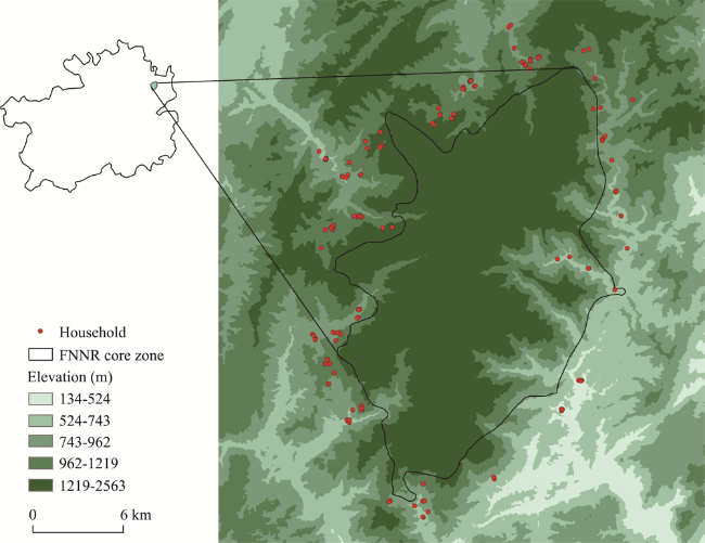
Table 4 Results of non-spatial and spatial (ESF) models for probability of enrolling in GTGP

Number of observations: 435. Bold indicates change of significance level from significant at 5% level to not significant at 5% level.
Eigenvectors are selected through a forward stepwise procedure with candidates selected based on Moran's Im/Moran's Imax >0.25 for positive spatial autocorrelation and Moran's I m/Moran's Imin >0.25 for negative spatial autocorrelation. Model 5 utilizes eigenvectors selected from the stepwise procedure (EV9, EV4, EV6, EV10) while Model 6 adds EV17.

It is interesting, moreover, that some independent variables change in significance levels, with three crossing the 0.05 α level from statistically significant to only marginally significant when comparing the basic model with the model incorporating ESF filtering ( Table 4). First, with regard to the concurrent PES variable, FEBC land area is a significant, negative predictor for enrollment in GTGP (p = 0.033) in the non-spatial model, but becomes insignificant in the models with ESF variables when the neighborhood size is 6 km (p = 0.067). While many socioeconomic and demographic variables have slightly different effects when neighborhood impacts are accounted for with varying neighborhood sizes, it is only gender (p= 0.045 in the non-spatial model) and household size (p= 0.019) which each also becoming only marginally significant in one of the six versions of the spatial FELRM. This is true of gender in Model 6 when the neighborhood size is 0.1 km (p = 0.053), while the coefficient of household size becomes insignificant only when the neighborhood size is very small at 0.02 km (Model 4, p = 0.083). An examination of all of the changes in p-values between the ESF filter variations and the basic non-spatial models finds the following: for Model 4 (only extremely close neighbors), five variables improve p-values, but household size is much weaker; in Model 5 (close neighbors), three are slightly better (lower p-value), two slightly worse (higher p-value), little change; in Model 6, with one more eigenvector added, 4 have better p’s, four worse including gender; Model 7 with medium size definition of neighborhood, 6 have betterp’s, including all three of the “switch” variables (FEBC, gender, household size), and only 2 lowerp’s, with the overall AIC highest of all the spatial models; while for both the much larger areal definitions of neighborhood, Models 8 and 9 based on radiuses of 5 km and 6 km, the number of variables with betterp’s is one less than those with weakerp-values.

4.3 Spatial autocorrelation

To further explore spatial autocorrelation of independent variables and model residuals, we calculated Moran’s I andp-value of residuals (Tables 3 and 5) and of independent variables (Table 6) for both the spatial and non-spatial models with the corresponding contiguity matrix.
Table 5 Results of Moran’s test for deviance residuals in the models ofTable 4
Model (Neighborhood) Contiguity matrix Moran's I Expected I Variance z-score p-value
Model 2 (0.02 km NB) Neighbors within 0.02 km -0.502 -0.003 0.040 -2.485 0.013
Model 4 (0.02 km NB) Neighbors within 0.02 km 0.118 0.206 0.035 -0.471 0.637
Model 2 (0.1 km NB) Neighbors within 0.1 km 0.134 -0.004 0.001 3.790 0.000
Model 5 (0.1 km NB) Neighbors within 0.1 km 0.099 -0.023 0.001 3.545 0.000
Model 6 (0.1 km NB) Neighbors within 0.1 km -0.026 -0.025 0.001 -0.019 0.985
Model 2 (0.5 km NB) Neighbors within 0.5 km 0.093 -0.003 0.000 4.378 0.000
Model 7 (0.5 km NB) Neighbors within 0.5 km -0.077 -0.032 0.000 -2.542 0.011
Model 2 (5 km NB) Neighbors within 5 km 0.014 -0.003 0.000 2.441 0.015
Model 8 (5 km NB) Neighbors within 5 km -0.003 -0.007 0.000 0.705 0.481
Model 2 (6 km NB) Neighbors within 6 km 0.013 -0.003 0.000 2.639 0.008
Model 9 (6 km NB) Neighbors within 6 km -0.014 -0.007 0.000 -1.467 0.142

Bold numbers indicate Moran’s I significant at 5% level.

Table 6 Results of Moran’s test for independent variables
Variable Neighbors within 0.02 km Neighbors within 0.1 km Neighbors within 0.5 km
Moran’s I z-score p-value Moran’s I z-score p-value Moran’s I z-score p-value
GTGP payment -0.004 -0.009 0.993 0.005 0.169 0.866 0.003 0.186 0.853
GTGP duration 0.134 1.005 0.315 -0.030 -0.648 0.517 -0.014 -0.442 0.658
Economic trees 0.003 0.040 0.968 0.025 0.631 0.528 0.005 0.278 0.781
Ecological plants -0.095 -0.684 0.494 0.078 1.883 0.060 0.011 0.484 0.628
Neighbors participating -0.141 -1.023 0.306 -0.026 -0.558 0.577 -0.023 -0.782 0.434
FEBC land area -0.487 -3.585 0.000 0.182 4.337 0.000 0.190 7.163 0.000
Age 0.487 3.617 0.000 0.054 1.315 0.188 -0.003 -0.023 0.982
Gender -0.028 -0.192 0.848 -0.056 -1.267 0.205 -0.096 -3.513 0.000
Education -0.010 -0.055 0.956 0.026 0.678 0.498 0.094 3.589 0.000
Annual agricultural expenses 0.049 0.384 0.701 0.058 1.446 0.148 0.221 8.430 0.000
Local off-farm income 0.138 1.046 0.296 0.028 0.712 0.477 -0.083 -3.023 0.003
Household size 0.329 2.454 0.014 0.097 2.353 0.019 0.137 5.172 0.000
Non-GTGP land 0.277 2.067 0.039 0.159 3.798 0.000 0.242 9.089 0.000
Variable Neighbors within 5 km Neighbors within 6 km
Moran’s I z-score p-value Moran’s I z-score p-value
GTGP payment 0.001 0.321 0.748 0.001 0.362 0.717
GTGP duration -0.014 -1.339 0.181 -0.013 -1.331 0.183
Economic trees 0.008 1.117 0.264 0.003 0.603 0.547
Ecological plants 0.009 1.285 0.199 0.005 0.934 0.350
Neighbors participating 0.001 0.370 0.712 0.000 0.314 0.754
FEBC land area 0.112 12.653 0.000 0.063 8.185 0.000
Age -0.021 -2.022 0.043 -0.017 -1.804 0.071
Gender 0.058 6.660 0.000 0.062 7.981 0.000
Education 0.007 1.009 0.313 0.000 0.248 0.804
Annual agricultural expenses 0.118 13.472 0.000 0.114 14.577 0.000
Local off-farm income -0.021 -2.111 0.035 -0.016 -1.681 0.093
Household size 0.047 5.492 0.000 0.073 9.332 0.000
Non-GTGP land 0.118 13.311 0.000 0.138 17.419 0.000

Bold numbers indicate Moran’s I significant at 5% level.

There are positive spatial autocorrelations in the residuals of the non-spatial model when the contiguity matrix are neighbors within 0.1 km (Moran’s I = 0.134,p < 0.001), 0.5 km (Moran’s I = 0.093, p < 0.001), 5 km (Moran’s I = 0.014, p = 0.015), and 6 km (Moran’s I = 0.013,p= 0.008), and negative spatial autocorrelations when the neighborhood size is 0.02 km (Moran’s I = -0.502,p = 0.013) (Table 3). After incorporating the ESF method, no significant spatial autocorrelations are detected in the residuals of spatial models with respect to the neighborhood sizes of 0.02 km (Model 4, Moran’s I = 0.118,p=0.637), 0.1 km (Model 6, Moran’s I = -0.026,p=0.985), 5 km (Model 8, Moran’s I = -0.003,p=0.481), and 6 km (Model 9, Moran’s I = -0.014,p=0.142) (Table 5). The results indicate that the selected eigenvectors in these four models control spatial autocorrelation well.
There is significant spatial autocorrelation in spatial Model 5 (Moran’s I = 0.099,p < 0.001), but this becomes insignificant in Model 6 when a fifth eigenvector (EV17) is added stepwise. We also tried incorporating various eigenvectors for the spatial ESF model of 0.1 km neighborhood size (Supplementary Tables S1 and S2), and found that Models 10, 11 and 12, which had fewer than the top 17 eigenvectors (Supplementary Table S1), had a significant level of positive spatial autocorrelation in the residuals (indicated by high positive z-scores in Supplementary Table S3), while Models 13, 14, 15 and 16 (Supplementary Table S2), which incorporated the top 17 or more eigenvectors, had a significant level of negative spatial autocorrelation (indicated by negative z-scores with p<0.05 in Supplementary Table S3). The results suggest that EV17 is the turning point for the significant positive and negative spatial autocorrelation in the residuals, and accounts for most of the spatial autocorrelation in Model 6.
Table S1 Results of non-spatial and spatial models with neighbors within 0.1 km for probability of enrolling in GTGP (with fewer than the top 17 eigenvectors)
Model 2 Model 10 Model 11 Model 12
Neighborhood size Non-spatial Neighbors within
0.1 km
Neighbors within
0.1 km
Neighbors within
0.1 km
Number of eigenvectors 0 14 15 16
Eigenvectors NA EV1-EV14 EV1-EV15 EV1-EV16
Coef. p-value VIF Coef. p-value VIF Coef. p-value VIF Coef. p-value VIF
(Intercept) -1.544 0.089 -1.352 0.168 -1.079 0.278 -1.628 0.138
GTGP payment 4.878 <0.001 1.035 5.035 <0.001 1.046 5.217 <0.001 1.055 5.859 <0.001 1.053
GTGP duration 0.008 0.816 1.048 -0.015 0.686 1.091 -0.018 0.616 1.097 -0.019 0.629 1.098
Economic trees 0.638 0.015 1.430 0.719 0.009 1.455 0.726 0.009 1.465 0.850 0.004 1.464
Ecological plants 0.100 0.713 1.415 0.085 0.766 1.441 0.152 0.599 1.477 0.181 0.557 1.473
Neighbors participating 1.626 0.006 1.035 1.680 0.006 1.048 1.708 0.006 1.052 2.037 0.002 1.053
FEBC land area -0.159 0.033 1.199 -0.190 0.017 1.311 -0.191 0.017 1.314 -0.224 0.008 1.315
Age 0.025 0.009 1.129 0.027 0.013 1.366 0.025 0.026 1.380 0.030 0.013 1.408
Gender -0.668 0.045 1.179 -0.509 0.164 1.296 -0.608 0.103 1.339 -0.605 0.138 1.436
Education -0.109 0.001 1.210 -0.143 <0.001 1.335 -0.158 <0.001 1.428 -0.162 <0.001 1.444
Annual agricultural expenses -0.556 <0.001 1.196 -0.494 0.001 1.254 -0.486 0.002 1.257 -0.431 0.009 1.266
Local off-farm income 0.037 0.002 1.259 0.044 <0.001 1.394 0.046 <0.001 1.418 0.045 0.001 1.427
Household size -0.204 0.019 1.282 -0.224 0.020 1.492 -0.258 0.009 1.569 -0.267 0.010 1.595
Non-GTGP land 0.086 0.011 1.225 0.087 0.018 1.325 0.091 0.013 1.331 0.099 0.011 1.332
AIC 543.18 541.01 539.74 539.48

Number of observations: 435. Bold indicates change of significance level from significant at 5% level to not significant at 5% level

Table S2 Results of non-spatial and spatial models with neighbors within 0.1 km for probability of enrolling in GTGP (with the top 17 or more eigenvectors)
Model 2 Model 13 Model 14
Neighborhood size Non-spatial Neighbors within 0.1 km Neighbors within 0.1 km
Number of eigenvectors 0 17 18
Eigenvectors NA EV1-EV17 EV1-EV18
Coef. p-value VIF Coef. p-value VIF Coef. p-value VIF
(Intercept) -1.544 0.089 -0.806 0.428 -1.684 0.126
GTGP payment 4.878 <0.001 1.035 5.126 <0.001 1.082 5.888 <0.001 1.083
GTGP duration 0.008 0.816 1.048 -0.021 0.568 1.121 -0.013 0.738 1.129
Economic trees 0.638 0.015 1.430 0.713 0.010 1.520 0.842 0.005 1.517
Ecological plants 0.100 0.713 1.415 0.142 0.624 1.481 0.204 0.508 1.486
Neighbors participating 1.626 0.006 1.035 1.727 0.006 1.088 2.118 0.002 1.097
FEBC land area -0.159 0.033 1.199 -0.190 0.018 1.363 -0.250 0.004 1.429
Age 0.025 0.009 1.129 0.022 0.046 1.477 0.032 0.009 1.482
Gender -0.668 0.045 1.179 -0.752 0.054 1.423 -0.628 0.123 1.432
Education -0.109 0.001 1.210 -0.165 <0.001 1.451 -0.166 <0.001 1.470
Model 2 Model 13 Model 14
Neighborhood size Non-spatial Neighbors within 0.1 km Neighbors within 0.1 km
Number of eigenvectors 0 17 18
Eigenvectors NA EV1-EV17 EV1-EV18
Coef. p-value VIF Coef. p-value VIF Coef. p-value VIF
Annual agricultural expenses -0.556 <0.001 1.196 -0.502 0.001 1.270 -0.446 0.007 1.273
Local off-farm income 0.037 0.002 1.259 0.046 <0.001 1.428 0.046 <0.001 1.434
Household size -0.204 0.019 1.282 -0.274 0.006 1.558 -0.265 0.010 1.549
Non-GTGP land 0.086 0.011 1.225 0.090 0.014 1.365 0.092 0.019 1.373
AIC 543.18 497.92 497.27
Model 15 Model 16
Neighborhood size Neighbors within 0.1 km Neighbors within 0.1 km
Number of eigenvectors 19 20
Eigenvectors EV1-EV19 EV1-EV20
Coef. p-value VIF Coef. p-value VIF
(Intercept) -1.661 0.133 -1.411 0.211
GTGP payment 5.930 <0.001 1.085 6.059 <0.001 1.090
GTGP duration -0.013 0.745 1.134 -0.005 0.896 1.139
Economic trees 0.865 0.004 1.520 0.843 0.005 1.511
Ecological plants 0.238 0.444 1.490 0.213 0.498 1.463
Neighbors participating 2.150 0.001 1.101 2.016 0.003 1.097
FEBC land area -0.252 0.004 1.414 -0.293 0.001 1.457
Age 0.030 0.013 1.496 0.028 0.027 1.526
Gender -0.685 0.096 1.462 -0.648 0.117 1.450
Education -0.163 <0.001 1.475 -0.157 <0.001 1.468
Annual agricultural expenses -0.479 0.004 1.318 -0.459 0.009 1.356
Local off-farm income 0.046 <0.001 1.444 0.048 <0.001 1.476
Household size -0.261 0.012 1.558 -0.247 0.020 1.566
Non-GTGP land 0.097 0.014 1.373 0.082 0.042 1.373
AIC 497.5 487.28

Number of observations: 435. Bold numbers with asterisk indicate change of significance level from significant at 5% level to not significant at 5% level

Table S3 Results of Moran’s test for deviance residuals in the models of Tables S1 and S2
Model (Neighborhood) Contiguity matrix Eigenvectors Moran’s I Expected I Variance z-score p-value
Model 2 (non-spatial model) Neighbors within 0.1 km NA 0.134 -0.004 0.001 3.790 0.000
Model 10 (0.1 km NB) Neighbors within 0.1 km EV1-EV14 0.042 -0.072 0.001 4.382 0.000
Model 11 (0.1 km NB) Neighbors within 0.1 km EV1-EV15 0.031 -0.074 0.001 4.106 0.000
Model 12 (0.1 km NB) Neighbors within 0.1 km EV1-EV16 0.021 -0.077 0.001 3.829 0.000
Model 13 (0.1 km NB) Neighbors within 0.1 km EV1-EV17 -0.143 -0.079 0.001 -2.507 0.012
Model 14 (0.1 km NB) Neighbors within 0.1 km EV1-EV18 -0.148 -0.082 0.001 -2.629 0.009
Model 15 (0.1 km NB) Neighbors within 0.1 km EV1-EV19 -0.155 -0.084 0.001 -2.801 0.005
Model 16 (0.1 km NB) Neighbors within 0.1 km EV1-EV20 -0.194 -0.087 0.001 -4.303 0.000

4.4 Best-practice model

AIC is defined to account for changes in degrees of freedom (Burnham and Anderson, 2002), therefore lower AIC scores stand for better fit. So we chose Model 6 as our best model (Table 4), to use for, e.g., policy recommendations. Nevertheless, we recognize that different independent variables may be spatially autocorrelated at different neighborhood sizes, so in this study, we are not able to identify a single neighborhood size, and therefore a “best” model that solves all neighborhood impact issues (see discussion below) is presented.

5 Discussion

5.1 ESF accounting for neighborhood impacts at different ranges of distance

Spatial autocorrelation is detected in our study on population in China in some shorter (0.02 km, 0.1 km), moderate (0.5 km), and longer distance (5 km, 6 km) neighborhood sizes. The short neighborhood sizes (from 0.02 km to 0.1 km) reflect considerable interactions with (immediate) neighbors, within a walking time of just a few minutes, a nearby cluster of dwellings. Within such a short distance, villagers can communicate with each other conveniently and frequently, and are more likely to be affected by them. For the moderate neighborhood sizes from 0.1 km to 1 km, people will not interact with some people as much, yet may still be subject to similar environmental and geographical features such as topography and distances to (the same) schools, roads and markets. For longer distances of 5 km to 6 km as the crow flies, in the mountains, they may use different roads and off-farm work access, have children who go to different schools, be located on different hill/mountain sides, or differ in some attitudes and social norms. Thus, different substantive aspects of neighborhood impacts are likely to operate across different distances (see also Hawley, 1950; Bilsborrow et al., 1984). It is important to point out that these neighborhood impacts are likely to be even greater in most real world sites (Sullivan et al., 2017), especially larger ones, as the data used in this paper come from a subset of fairly similar low-income rural households in a single Chinese nature reserve in China.
The ESF method is useful since it can eliminate spatial autocorrelation that is inherent in human populations living close to each other at some neighborhood sizes (0.02 km, 0.1 km, 1 km, 5 km, and 6 km). Although spatial autocorrelation is significant at the neighborhood size of 0.5 km (in both the non-spatial and spatial models; Table 5), the p-value of Moran’s I for the ESF model increases compared to the non-spatial model, suggesting that we are less likely to reject the null hypothesis that the spatial distribution of feature values is the result of a random spatial process. We can learn from the Moran’s test of Models 5 and 6 that EV17 can explain most of the positive spatial autocorrelation when the neighborhood size is 0.1 km (Tables S1 and S2). The reason why there is a big difference in Moran’s I in models with and without this one eigenvector (EV17) may be the physical structure of the neighborhoods used here, which vary a lot from clusters of households horizontally close but vertically not close. For situations when all the polygons have at least one-point in common (Chun and Griffith, 2014; Xiao et al., 2017), eigenvalues change gradually from the largest to the smallest. For the FNNR dataset with different definitions of neighborhood, the neighbor structure is not fully connected, which means that a group of observations are not connected with other groups of observations based on a specific distance. As a result, the weight matrix has a block structure, and the eigenvector has nonzero values for one group and zeros for other groups, indicating that an eigenvector based on one neighborhood size specification may account for a high level of spatial autocorrelation among observations for some populations but not others, for which a different neighborhood specification may work better. Determining a priori an optimal general “neighborhood size” is risky as it may vary with topography, soil quality, population density, level of development, and cultural factors (how much space people feel they need varies).

5.2 Impacts of independent variables in non-spatial and spatial models

The results here for aspects of PES policy differ little in this study between the non-spatial model and the spatial models incorporating spatial filtering. This suggests that there are no particular neighborhood differences in these policy choice variables, which is not surprising given the similarities in the characteristics of the populations of the various clusters (low-income rural households, minority populations, mountainous terrain, much out-migration, etc.). Of course, it is not surprising to find that once controlling for other variables, the social norm (represented as the percentage of neighbors expected to participate in GTGP) is a significant, positive predictor of a household’s willingness to participate in GTGP regardless of neighborhood size. One previous study similarly found that when neighbors anticipated reconverting land enrolled in GTGP back to agriculture from forest once the PES program ends, so did the household under study (Chenet al., 2009). Thus, households who live in the same community have many opportunities to interact, which fosters and maintains social norms, including motivations to sign up for GTGP, or abandon it.
Significance levels of involvement in a concurrent PES program and some socioeconomic and demographic variables may change when neighborhood impacts are taken into account through filtering out spatial autocorrelation using the ESF method. While a few earlier studies used the ESF method to eliminate spatial autocorrelation in regression residuals, they did not detect changes in the significance levels of independent variables (Chun and Griffith, 2011; Xiao et al., 2017). Similarly, in this study only a few variables’ significance levels changed when different neighborhood sizes were used. The area of forest enrolled in a concurrent FEBC program has a significantly negative effect in the non-spatial model, likely due to the FEBC program increasing farmer’s incomes and making them less dependent on the incentives of the GTGP program (Zhanget al., 2018b). In addition, in FNNR participants reported needing to spend time safeguarding their FEBC land to avoid forest fires and theft, which may have weakened motivations to enroll in the GTGP program and have to plant and care for economic or ecological trees (Yost et al., 2020). We found there is spatial autocorrelation in the variable FEBC land area at all detected neighborhood sizes (Table 6) but its significance level changes from significant to insignificant only at the largest neighborhood size of 6 km in the ESF model (Table 4). This may suggest that a large neighborhood may involve some households with very different characteristics and sizes of forestland. As a result, the spatial dimension of the FEBC variable might lose its effects on local people’s intensions to enroll or not in GTGP. However, even here, as thep-value (0.067) just barely crosses the 0.05 threshold, there is no basis for totally rejecting the result that FEBC area (and the resulting household income it generates) is negatively linked to the probability of enrolling in GTGP, even after controlling for spatial autocorrelation.
The influence of gender on household participation in PES program has been observed to vary across studies (Stevens et al., 1999; Zbinden and Lee, 2005; Chen et al., 2009; Chen et al., 2012; Kaczan et al., 2013; Chen et al., 2017). In our study site, the coefficient for gender of respondent has been found invariably negative, that is, female-headed households are less likely to enroll in GTGP. This can be thought of as arising from women heads’ thinking that they have fewer opportunities to get involved in local off-farm work so need to keep their land to farm for food security. The coefficient of gender varies as does its significance level by neighborhood size (Table 4), but the effect is generally quite strong for all neighborhood sizes used in the ESF models. In the non-spatial model, its significance level is p=0.045, which falls only slightly to 0.053 in Model 6 at the neighborhood size of 0.1 km but has better p-values (lower) than 0.045 at all other neighborhood sizes (and lowest in Model 7 at 0.5 km at p = 0.009). The size of its coefficient is fairly stable, from -0.7 to -1.0, indicating a strong effect.
Similarly, there is evidence on how neighborhood size affects the roles of socioeconomic variables. At the larger neighborhood sizes (0.1 km, 0.5 km, 5 km and 6 km), households of larger size (more members) are found to be more reluctant to participate in GTGP. This effect is insignificant at the smallest neighborhood size (0.02 km), with the p value switching from 0.019 (non-spatial model) to 0.083 and less significance in the spatial model. What might cause this? Perhaps at such a small neighborhood size, it is very common for individuals to communicate with neighbors on issues related to participating in the GTGP, making household size not relevant.
Finally, are there differences in the effects of neighborhood size on the effects of the variable non-GTGP land (or land not yet enrolled in GTGP) on the enrolment of (additional) farmland in GTGP? As hypothesized, this variable is positively linked to the GTGP enrollment decision in the non-spatial and all spatial ESF models, regardless of neighborhood size. Having more available non-GTGP land provides a wider variety of options for land use, such as continuing to grow crops even with participation in GTGP (Chen et al., 2009; Chen et al., 2012). This is also consistent with common sense as more available non-GTGP land should alleviate concerns about household food security (Wandersee et al., 2012; Liu et al., 2014; Wang et al., 2019), at the same time as some land may already be enrolled in GTGP, modestly contributing to income (Liu et al., 2008; Yin et al., 2014; Wang et al., 2017). Thez-scores of Moran’s I for both household size and non-GTGP land are greater than 1.96 at all distances, with Moran’s I larger than zero and increasing dramatically with size of neighborhood (as for household size), which suggests that there is positive spatial autocorrelation at all neighborhood sizes for these two variables. One reason for this spatial autocorrelation might be that household size and non-GTGP land are fairly homogeneous even over large areas in rural China. This is likely for several reasons. First, the one-child policy, terminated in 2015 only after the survey data were collected (Deng et al., 2016), has led to very similar and small family sizes, making household size vary little across space. Similarly, the total area of land allocated via long-term lease to rural households (including nearby and within FNNR) in the opening-up period in the 1980s varied very little as land in government collective (communal) farms was simply divided up among the local commune member households (Lin, 1987).
In sum, when we incorporate the ESF method at different neighborhood sizes, significance levels of household size, gender, and FEBC land area change from significant to insignificant at neighborhood sizes of 0.02 km, 0.5 km, and 6 km, respectively. Overall, we posit that the selected ESFs capture more heterogeneity and (relatively) more local spatial differentiation at these neighborhood sizes compared to the other sizes. Further research might help determine reasons for these spatial differences. Also worthy of mention is that our results are not much dependent on the way we define neighborhood. For instance, we selected neighborhoods based on the Queen’s or Rook’s definitions at the first, second, … up to the fifth orders. The corresponding results (Supplementary Tables S4, S5, S6 and S7) are largely consistent with the ones above.
Table S4 Comparison for the non-spatial model, best-practice model, and Rook 3rd order ESF model: dependent variable, probability of enrolling in GTGP
Model 2 Model 6 Model 24
Contiguity Non-spatial Neighbors within 0.1 km Rook 3rd order
Number of candidate eigenvectors for stepwise procedure NA 12 16
Number of eigenvectors 0 5 4
Eigenvectors NA EV9, EV4, EV6,
EV10, EV17
EV16, EV2, EV10, EV5
Coef. p-value VIF Coef. p-value VIF Coef. p-value VIF
(Intercept) -1.544 0.089 -2.239 0.027 -1.028 0.288
GTGP payment 4.878 <0.001 1.035 5.571 <0.001 1.057 4.422 0.001 1.036
GTGP duration 0.008 0.816 1.048 -0.002 0.959 1.084 -0.006 0.877 1.065
Economic trees 0.638 0.015 1.430 0.748 0.008 1.490 0.590 0.028 1.424
Ecological plants 0.1 0.713 1.415 0.087 0.766 1.455 -0.070 0.805 1.425
Neighbors participating 1.626 0.006 1.035 1.791 0.004 1.053 1.597 0.009 1.038
FEBC land area -0.159 0.033 1.199 -0.180 0.021 1.231 -0.169 0.031 1.248
Age 0.025 0.009 1.129 0.034 0.001 1.240 0.022 0.032 1.185
Gender -0.668 0.045 1.179 -0.713 0.053 1.259 -0.577 0.093 1.200
Education -0.109 0.001 1.210 -0.100 0.008 1.278 -0.100 0.006 1.290
Annual agricultural expenses -0.556 <0.001 1.196 -0.504 0.002 1.221 -0.598 <0.001 1.267
Local off-farm income 0.037 0.002 1.259 0.039 0.002 1.309 0.041 0.001 1.233
Household size -0.204 0.019 1.282 -0.201 0.032 1.346 -0.248 0.008 1.355
Non-GTGP land 0.086 0.011 1.225 0.091 0.011 1.267 0.117 0.002 1.365
AIC 543.18 506.44 527.84

Number of observations: 435. Bold indicates change of significance level from significant at 5% level to not significant at 5% level.
We first generated eigenvectors for Queen and Rook 1st to 5th order contiguity and cooperated with the FELRM using stepwise procedure respectively (Tables S5 and S6). We calculated Moran’s I andp-value for each model (Table S7). There are spatial autocorrelations detected in the non-spatial models with 1st order queen contiguity, 2nd order queen contiguity, 3rd order queen contiguity, 1st order rook contiguity, 2nd order rook contiguity, 3rd order rook contiguity, 4th order rook contiguity, and 5th order rook contiguity. ESF method can account the spatial autocorrelations properly for these models (Table S7). Model 24 has the highest p-value for Moran’s I compared to other Queen and Rook ESF models. The best-practice model (Model 6) has the lowest AIC score and highest Moran’s Ip-value compared to other distance based ESF models.

Table S5 Results of non-spatial and spatial (Queen 1st-5th order) models for probability of enrolling in GTGP
Model 2 Model 17 Model 18
Contiguity Non-spatial Queen 1st order Queen 2nd order
Number of candidate
eigenvectors for
stepwise procedure
NA 29 18
Number of eigenvectors 0 19 4
Eigenvectors NA EV16, EV31, EV40, EV34, EV28, EV38, EV2, EV5, EV39, EV22, EV35, EV18, EV19, EV10, EV24, EV6, EV25, EV13, EV4 EV16, EV2, EV10, EV5
Coef. p-value VIF Coef. p-value VIF Coef. p-value VIF
(Intercept) -1.544 0.089 -0.65 0.551 -1.028 0.288
GTGP payment 4.878 <0.001 1.035 6.005 <0.001 1.102 4.422 0.001 1.036
GTGP duration 0.008 0.816 1.048 0.015 0.709 1.156 -0.006 0.877 1.065
Model 2 Model 17 Model 18
Contiguity Non-spatial Queen 1st order Queen 2nd order
Number of candidate
eigenvectors for
stepwise procedure
NA 29 18
Number of eigenvectors 0 19 4
Eigenvectors NA EV16, EV31, EV40, EV34, EV28, EV38, EV2, EV5, EV39, EV22, EV35, EV18, EV19, EV10, EV24, EV6, EV25, EV13, EV4 EV16, EV2, EV10, EV5
Coef. p-value VIF Coef. p-value VIF Coef. p-value VIF
Economic trees 0.638 0.015 1.430 0.657 0.024 1.478 0.59 0.028 1.424
Ecological plants 0.1 0.713 1.415 0.095 0.759 1.511 -0.07 0.805 1.425
Neighbors participating 1.626 0.006 1.035 1.362 0.039 1.083 1.597 0.009 1.038
FEBC land area -0.159 0.033 1.199 -0.326 <0.001 1.490 -0.169 0.031 1.248
Age 0.025 0.009 1.129 0.022 0.058 1.331 0.022 0.032 1.185
Gender -0.668 0.045 1.179 -0.653 0.103 1.425 -0.577 0.093 1.200
Education -0.109 0.001 1.210 -0.154 <0.001 1.454 -0.1 0.006 1.290
Annual agricultural expenses -0.556 <0.001 1.196 -0.449 0.009 1.460 -0.598 <0.001 1.267
Local off-farm income 0.037 0.002 1.259 0.056 <0.001 1.423 0.041 0.001 1.233
Household size -0.204 0.019 1.282 -0.364 0.001 1.616 -0.248 0.008 1.355
Non-GTGP land 0.086 0.011 1.225 0.127 0.002 1.454 0.117 0.002 1.365
AIC 543.18 509.58 527.84
Model 19 Model 20 Model 21
Contiguity Queen 3rd order Queen 4th order Queen 5th order
Number of candidate eigenvectors for stepwise procedure 10 9 8
Number of eigenvectors 4 4 4
Eigenvectors EV5, EV4, EV2, EV6 EV5, EV4, EV2, EV6 EV5, EV4, EV2, EV6
Coef. p-value VIF Coef. p-value VIF Coef. p-value VIF
(Intercept) -1.363 0.148 -1.368 0.146 -1.371 0.145
GTGP payment 5.049 <0.001 1.047 5.049 <0.001 1.047 5.048 <0.001 1.047
GTGP duration 0.005 0.887 1.057 0.005 0.897 1.058 0.004 0.901 1.058
Economic trees 0.59 0.027 1.434 0.591 0.026 1.434 0.591 0.026 1.433
Ecological plants 0.093 0.739 1.427 0.095 0.733 1.426 0.096 0.73 1.426
Neighbors participating 1.58 0.009 1.047 1.589 0.008 1.047 1.595 0.008 1.048
FEBC land area -0.167 0.029 1.216 -0.165 0.03 1.215 -0.164 0.031 1.214
Age 0.026 0.01 1.158 0.026 0.009 1.158 0.026 0.009 1.157
Gender -0.74 0.03 1.224 -0.738 0.031 1.223 -0.736 0.031 1.222
Education -0.119 0.001 1.251 -0.119 0.001 1.250 -0.119 0.001 1.250
Annual agricultural expenses -0.477 0.001 1.217 -0.475 0.001 1.220 -0.475 0.001 1.222
Local off-farm income 0.041 0.001 1.302 0.041 0.001 1.304 0.041 0.001 1.305
Household size -0.296 0.001 1.424 -0.299 0.001 1.428 -0.3 0.001 1.431
Non-GTGP land 0.111 0.002 1.340 0.11 0.003 1.336 0.109 0.003 1.334
AIC 538.44 538.44 538.08

Number of observations: 435.

Table S6 Results of non-spatial and spatial (Rook 1st-5th order) models for probability of enrolling in GTGP
Model 2 Model 22 Model 23
Contiguity Non-spatial Rook 1st order Rook 2nd order
Number of candidate eigenvectors for stepwise procedure NA 43 18
Number of Eigenvectors 0 19 4
Eigenvectors NA EV16, EV31, EV40, EV34, EV28, EV38, EV2, EV5, EV39, EV22, EV35, EV18, EV19, EV10, EV24, EV6, EV25, EV13, EV4 EV16, EV2, EV10, EV5
Coef. p-value VIF Coef. p-value VIF Coef. p-value VIF
(Intercept) -1.544 0.089 -0.65 0.551 -1.068 0.269
GTGP payment 4.878 <0.001 1.035 6.005 <0.001 1.102 4.392 0.001 1.036
GTGP duration 0.008 0.816 1.048 0.015 0.709 1.156 -0.006 0.876 1.066
Economic trees 0.638 0.015 1.430 0.657 0.024 1.478 0.593 0.027 1.423
Ecological plants 0.1 0.713 1.415 0.095 0.759 1.511 -0.06 0.831 1.423
Neighbors participating 1.626 0.006 1.035 1.362 0.039 1.083 1.601 0.009 1.039
FEBC land area -0.159 0.033 1.199 -0.326 <0.001 1.490 -0.168 0.032 1.249
Age 0.025 0.009 1.129 0.022 0.058 1.331 0.022 0.028 1.180
Gender -0.668 0.045 1.179 -0.653 0.103 1.425 -0.595 0.083 1.198
Education -0.109 0.001 1.210 -0.154 <0.001 1.454 -0.1 0.006 1.288
Annual agricultural expenses -0.556 <0.001 1.196 -0.449 0.009 1.460 -0.597 <0.001 1.268
Local off-farm income 0.037 0.002 1.259 0.056 <0.001 1.423 0.04 0.001 1.237
Household size -0.204 0.019 1.282 -0.364 0.001 1.616 -0.242 0.009 1.355
Non-GTGP land 0.086 0.011 1.225 0.127 0.002 1.454 0.116 0.002 1.361
AIC 543.18 509.58 528.8
Model 24 Model 25 Model 26
Contiguity Rook 3rd order Rook 4th order Rook 5th order
Number of candidate eigenvectors for stepwise procedure 16 15 15
Number of Eigenvectors 4 5 4
Eigenvectors EV16, EV2, EV10, EV5 EV2, EV5, EV10, EV14, EV6 EV2, EV5, EV10, EV14
Coef. p-value VIF Coef. p-value VIF p-value p-value VIF
(Intercept) -1.028 0.288 -1.324 0.158 -1.433 0.123
GTGP payment 4.422 0.001 1.036 4.822 <0.001 1.041 4.727 0.001 1.037
GTGP duration -0.006 0.877 1.065 0.003 0.934 1.058 0.003 0.942 1.057
Economic trees 0.59 0.028 1.424 0.574 0.031 1.429 0.598 0.024 1.425
Ecological plants -0.07 0.805 1.425 0.039 0.889 1.416 0.029 0.916 1.416
Neighbors participating 1.597 0.009 1.038 1.518 0.011 1.042 1.572 0.009 1.039
FEBC land area -0.169 0.031 1.248 -0.152 0.049 1.215 -0.147 0.055 1.209
Age 0.022 0.032 1.185 0.025 0.011 1.147 0.026 0.008 1.140
Gender -0.577 0.093 1.200 -0.642 0.059 1.201 -0.609 0.072 1.184
Education -0.1 0.006 1.290 -0.119 0.001 1.290 -0.116 0.001 1.281
Annual agricultural expenses -0.598 <0.001 1.267 -0.497 0.001 1.234 -0.519 0.001 1.227
Local off-farm income 0.041 0.001 1.233 0.038 0.001 1.254 0.038 0.002 1.254
Household size -0.248 0.008 1.355 -0.255 0.006 1.391 -0.243 0.008 1.372
Non-GTGP land 0.117 0.002 1.365 0.103 0.005 1.348 0.102 0.005 1.353
AIC 527.84 538.92 538.9

Number of observations: 435. Bold indicates change of significance level from significant at 5% level to not significant at 5% level.

Table S7 Results of Moran’s test for deviance residuals in the models of Tables S5 and S6
Model (Neighborhood) Contiguity matrix Moran’s I Expected I Variance Z-score p-value
Model 2 (Queen 1st order) Queen 1st order 0.034 -0.005 0.000 2.611 0.009
Model 17 (Queen 1st order) Queen 1st order -0.055 -0.032 0.000 -1.906 0.057
Model 2 (Queen 2nd order) Queen 2nd order 0.022 -0.004 0.000 3.147 0.002
Model 18 (Queen 2nd order) Queen 2nd order -0.004 -0.009 0.000 0.658 0.511
Model 2 (Queen 3rd order) Queen 3rd order 0.007 -0.003 0.000 2.117 0.034
Model 19 (Queen 3rd order) Queen 3rd order -0.007 -0.003 0.000 -0.752 0.452
Model 2 (Queen 4th order) Queen 4th order 0.004 -0.003 0.000 1.377 0.169
Model 20 (Queen 4th order) Queen 4th order -0.010 -0.003 0.000 -1.357 0.175
Model 2 (Queen 5th order) Queen 5th order 0.002 -0.003 0.000 1.036 0.300
Model 21 (Queen 5th order) Queen 5th order -0.011 -0.003 0.000 -1.625 0.104
Model 2 (Rook 1st order) Rook 1st order 0.034 -0.005 0.000 2.611 0.009
Model 22 (Rook 1st order) Rook 1st order -0.055 -0.032 0.000 -1.906 0.057
Model 2 (Rook 2nd order) Rook 2nd order 0.022 -0.004 0.000 3.147 0.002
Model 23 (Rook 2nd order) Rook 2nd order -0.004 -0.009 0.000 0.637 0.524
Model 2 (Rook 3rd order) Rook 3rd order 0.019 -0.004 0.000 2.867 0.004
Model 24 (Rook 3rd order) Rook 3rd order -0.005 -0.009 0.000 0.524 0.601
Model 2 (Rook 4th order) Rook 4th order 0.018 -0.004 0.000 2.750 0.006
Model 25 (Rook 4th order) Rook 4th order -0.001 -0.010 0.000 1.399 0.162
Model 2 (Rook 5th order) Rook 5th order 0.018 -0.004 0.000 2.686 0.007
Model 26 (Rook 5th order) Rook 5th order 0.001 -0.009 0.000 1.446 0.148

Bold numbers indicate Moran’s I significant at 5% level.

6 Conclusions

In this article, we have modeled the determinants of household participation in PES programs in a case study in Guizhou province of China, with a focus on how to control neighborhood or contextual effects. Alternative neighborhood sizes were used to control neighborhood impacts on coefficients in a standard fixed effects logistic regression model (FELRM). We found that once spatial autocorrelation (owing to neighborhood effects) is suitably accounted for, several more reasonable coefficients and significance levels are obtained but tend to differ according to neighborhood size. Therefore, not accounting for neighborhood impacts may often lead to biased parameter estimates and even improper conclusions. This issue has been largely overlooked so far in this literature, particularly with reference to studies on the impacts of PES policies. In this study, the eigenvector spatial filtering (ESF) method is shown to be effective in controlling spatial autocorrelation in the analysis of spatial data. Therefore, we recommend the ESF method be considered an effective way to control neighborhood impacts and thereby reduce bias in estimates of parameters and improve inferences about causation and policy effects.
The study here also makes substantive contributions to the PES and conservation literatures in several respects. First, there has been little previous work investigating neighborhood impacts on household decisions to participate in PES programs. Our analysis shows that examining such impacts may uncover mechanisms underlying PES participation (and more broadly, any decisions involving spatially referenced data) that are otherwise undetectable. This can help planners, policymakers, and researchers take into account community interests and/or spatial features in the PES programs prior to seeking to enroll households. Second, we observe that different kinds of neighborhood impacts may exist at different neighborhood sizes, so a one-scale-fits-all approach may not work well. Indeed, researchers should seek to identify differences in neighborhood size impacts based on theory in the field of study pertaining to the variables being studied and/or data-mining (experimenting with different neighborhood sizes). In our study, we mainly used the latter but sought to offer theory-based interpretations for different neighborhood size effects detected. Last but not least, our data-mining approach can be used to explore the effects of different sizes of neighborhoods, a theoretically and empirically important topic in many fields of social science, for example, in sociology, demography, and public health (Medina et al., 2013; Zvoleff et al., 2013; Liu and Shen, 2017), as well as in environmental studies such as the present one.
Our approach here may be viewed by some as only a more complex alternative to the more standard fixed effects model. Such a model incorporates a set of dummy variables with one for each spatial unit (neighborhood or community) to control contextual differences to obtain more unbiased estimates of parameters at lower (e.g., household and individual) levels. But the fixed effects approach is statistically inefficient in costing degrees of freedom in the estimation (if k= number of communities, then k-1 degrees of freedom are lost). As our approach does not need any prior knowledge about neighborhood size, it can complement the usual multilevel model (or a random effects) approach, which needs to know the grouping of higher level units beforehand (e.g., administrative units, spatial regions). It can be used to explore at what size a particular neighborhood is most relevant for a certain topic—viz., smaller areas within which local people influence each another in decisions related to purchasing foods or children walking to a primary school, larger ones for health care, older children attending secondary schools, and even larger ones for employment involving commuting to work (Hawley, 1950; Bilsborrow et al., 1984). Neighborhood size is also a key factor to consider in environmental conservation and natural resources management. Spatial effects are likely for many variables at some neighborhood size, and a one- size-fits-all management policy and implementation measure is likely to be inefficient. It is important for policymakers to develop (for example) infrastructure location/management plans that vary with the type of infrastructure and service. We hope that this research will not only lead to a greater recognition of the importance of neighborhood effects in PES and other conservation decisions, but also provide a practical, data-mining based approach that helps other researchers and planners address these effects.

This research was funded by the National Science Foundation under the Dynamics of Coupled Natural and Human Systems program [Grant DEB-1212183 and BCS-1826839]. This research also received financial and research support from San Diego State University. We thank Fanjingshan National Nature Reserve in China and the Research Center for Eco-Environmental Sciences at the Chinese Academy of Sciences. The collaboration of Bilsborrow was supported by the Population Research Infrastructure Program grant (P2C, HD050924) to the Carolina Population Center at the University of North Carolina by the US National Institute of Child Health and Human Development. We would also like to thank the editor and anonymous reviewer for their insightful comments.

[1]
Adhikari B, Agrawal A, 2014. Understanding the social and ecological outcomes of PES projects: A review and an analysis. Conservation and Society, 11(4):359.

DOI

[2]
Adhikari B, Boag G, 2013. Designing payments for ecosystem services schemes: Some considerations. Current Opinion in Environmental Sustainability, 5(1):72-77.

DOI

[3]
An L, Tsou M H, Spitzberg B H et al., 2016. Latent trajectory models for space-time analysis: An application in deciphering spatial panel data. Geographical Analysis, 48(3):314-336.

DOI

[4]
An L, Mak J, Yang S et al., 2020. Cascading impacts of payments for ecosystem services in complex human-environment systems. Journal of Artificial Societies and Social Simulation, 23(5)

[5]
Balderas Torres A, MacMillan D C, Skutsch M et al., 2013. Payments for ecosystem services and rural development: Landowners’ preferences and potential participation in western Mexico. Ecosystem Services, 6:72-81.

DOI

[6]
Bendor J, Swistak P, 2001. The evolution of norms. American Journal of Sociology, 106(6):1493-1545.

DOI

[7]
Bilsborrow R E, 2016. Concepts, definitions and data collection approaches. In:International Handbook of Migration and Population Distribution. Dordrecht: Springer:109-156.

[8]
Bilsborrow R E, Oberai A S, Standing G, 1984. Migration Surveys in Low-income Countries: Guidelines for Survey and Questionnaire Design. London: Croom-Helm.

[9]
Bremer L L, Farley K A, Lopez-Carr D, 2014. What factors influence participation in payment for ecosystem services programs? An evaluation of Ecuador’s SocioPáramo program. Land Use Policy, 36:122-133.

DOI

[10]
Burden S, Cressie N, Steel D G, 2015. The SAR model for very large datasets: A reduced rank approach. Econometrics, 3(2):317-338.

DOI

[11]
Burnham K P, Anderson D R , 2002. Model Selection and Multimodel Inference. 2nd ed. Berlin: Springer.

[12]
Case A, 1992. Neighborhood influence and technological change. Regional Science and Urban Economics, 22(3):491-508.

DOI

[13]
Chen X, Lupi F, An L et al., 2012. Agent-based modeling of the effects of social norms on enrollment in payments for ecosystem services. Ecological Modelling, 229:16-24.

DOI

[14]
Chen X, Lupi F, He G et al., 2009. Linking social norms to efficient conservation investment in payments for ecosystem services. Proceedings of the National Academy of Sciences, 106(28):11812-11817.

DOI

[15]
Chen Y, Zhang Q, Liu W et al., 2017. Analyzing farmers’ perceptions of ecosystem services and PES schemes within Agricultural landscapes in Mengyin County, China: Transforming trade-offs into synergies. Sustainability, 9(8):1459.

DOI

[16]
Chun Y, 2008. Modeling network autocorrelation within migration flows by eigenvector spatial filtering. Journal of Geographical Systems, 10(4):317-344.

DOI

[17]
Chun Y, 2014. Analyzing space-time crime incidents using eigenvector spatial filtering: An application to vehicle burglary. Geographical Analysis, 46(2):165-184.

DOI

[18]
Chun Y, Griffith D A, 2011. Modeling network autocorrelation in space-time migration flow data: An eigenvector spatial filtering approach. Annals of the Association of American Geographers, 101(3):523-536.

DOI

[19]
Chun Y, Griffith D A, Lee M et al., 2016. Eigenvector selection with stepwise regression techniques to construct eigenvector spatial filters. Journal of Geographical Systems, 18(1):67-85.

DOI

[20]
Coleman J S, 1994. Foundations of Social Theory. Cambridge: Harvard University Press.

[21]
Darand M, Dostkamyan M, Rehmani M I A, 2017. Spatial autocorrelation analysis of extreme precipitation in Iran. Russian Meteorology and Hydrology, 42(6):415-424.

DOI

[22]
Deng S, Liu J, He X, 2016. Analysis of the advantages and disadvantages of the universal two-child policy in China. Industrial & Science Tribune, 15(4):7-8. (in Chinese)

[23]
Dietz R D, 2002. The estimation of neighborhood effects in the social sciences: An interdisciplinary approach. Social Science Research, 31(4):539-575.

DOI

[24]
Feng X, Fu B, Lu N et al., 2013. How ecological restoration alters ecosystem services: An analysis of carbon sequestration in China’s Loess Plateau. Scientific Reports, 3:3-7.

[25]
Feng X, Fu B, Piao S et al., 2016. Revegetation in China’s Loess Plateau is approaching sustainable water resource limits. Nature Climate Change, 6(11):1019-1022.

DOI

[26]
Fichet de Clairfontaine A, Fischer M M, Lata R et al., 2015. Barriers to cross-region research and development collaborations in Europe: Evidence from the fifth European framework programme. Annals of Regional Science, 54(2):577-590.

DOI

[27]
Foster A D, Rosenzweig M R, 1995. Learning by doing and learning from others: Human capital and technical change in agriculture. Journal of Political Economy, 103(6):1176-1209.

DOI

[28]
Gillenwater M, 2012. What is additionality? Part 3: Implications for stacking and unbundling. GHG Management Institute, Discussion Paper, (003)

[29]
Goodchild M F, 1986, Spatial autocorrelation. In: Concepts and Techniques in Modern Geography. Norwich: GeoBooks, 1986, No. 47.

[30]
Griffith D, Chun Y, Li B, 2019. Spatial Regression Analysis Using Eigenvector Spatial Filtering. Cambridge: Academic Press.

[31]
Griffith D A, 2000. A linear regression solution to the spatial autocorrelation problem. Journal of Geographical Systems, 2(2):141-156.

DOI

[32]
Griffith D A, 2003. Spatial Autocorrelation and Spatial Filtering: Gaining Understanding Through Theory and Scientific Visualization. Berlin: Springer-Verlag.

[33]
Griffith D A, Fischer M M, Lesage J P, 2017. The spatial autocorrelation problem in spatial interaction modelling: A comparison of two common solutions. Letters in Spatial and Resource Sciences, 10(1):75-86.

DOI

[34]
Guo G, Hipp J, 2004. Longitudinal analysis for continuous outcomes:Random effects models and latent trajectory models. In: Hardy M, Bryman A (eds.). New Handbook on Data Analysis. London: Sage,347-368.

[35]
Hawley A H, 1950. Human Ecology:A Theory of Community Structure. New York: Ronald Press,257.

[36]
Helbich M, Arsanjani J J, 2015. Spatial eigenvector filtering for spatiotemporal crime mapping and spatial crime analysis. Cartography and Geographic Information Science, 42(2):134-148.

DOI

[37]
Helbich M, Griffith D A, 2016. Spatially varying coefficient models in real estate: Eigenvector spatial filtering and alternative approaches. Computers, Environment and Urban Systems, 57:1-11.

DOI

[38]
I.W. H. E. Report, World Heritage Nomination-Iucn Technical Evaluation:1-34.

[39]
Jack B K, Kousky C, Sims K R, 2008. Designing payments for ecosystem services: Lessons from previous experience with incentive-based mechanisms. Proceedings of the National Academy of Sciences, 105(28):9465-9470.

[40]
Kaczan D, Swallow B M, Adamowicz W L V, 2013. Designing payments for ecosystem services (PES) program to reduce deforestation in Tanzania: An assessment of payment approaches. Ecological Economics, 95:20-30.

DOI

[41]
Lara E, Roussel-Delif L, Fournier B et al., 2016. Soil microorganisms behave like macroscopic organisms: Patterns in the global distribution of soil euglyphid testate amoebae. Journal of Biogeography, 43(3):520-532.

DOI

[42]
Layton D F, Siikamäki J, 2009. Payments for ecosystem services programs: Predicting landowner enrollment and opportunity cost using a beta-binomial model. Environmental and Resource Economics, 44(3):415-439.

DOI

[43]
Lee B A, Oropesa R S, Kanan J W, 1994. Neighborhood context and residential mobility. Demography, 31(2):249-270.

PMID

[44]
Li W, Chen J, Zhang Z, 2020. Forest quality-based assessment of the Returning Farmland to Forest Program at the community level in SW China. Forest Ecology and Management, 461:117938.

DOI

[45]
Li W, Zinda J A, Zhang Z, 2019. Does the “Returning Farmland to Forest Program” drive community-level changes in landscape patterns in China? Forests, 10(10):933.

DOI

[46]
Lin J Y, 1987. The household responsibility system reform in China: A peasant’s institutional choice. American Journal of Agricultural Economics, 69(2):410-415.

DOI

[47]
Liu J, Diamond J, 2005. China’s environment in a globalizing world. Nature, 435:1179-1186.

DOI

[48]
Liu J, Li S, Ouyang Z, Tam C et al., 2008. Ecological and socioeconomic effects of China’s policies for ecosystem services. Proceedings of the National Academy of Sciences, 105(28):9477-9482.

DOI

[49]
Liu Y, Fang F, Li Y, 2014. Key issues of land use in China and implications for policy making. Land Use Policy, 40:6-12.

DOI

[50]
Liu Y, Shen J, 2017. Modelling skilled and less-skilled interregional migrations in China, 2000-2005. Population, Space and Place, 23(4):e2027.

[51]
Long H L, Heilig G K, Wang J et al., 2006. Land use and soil erosion in the upper reaches of the Yangtze River: Some socio-economic considerations on China’s Grain-for-Green Programme. Land Degradation and Development, 17(6):589-603.

DOI

[52]
Lu G, Yin R, 2020. Evaluating the evaluated socioeconomic impacts of China’s sloping land conversion program. Ecological Economics, 177:106785.

DOI

[53]
Y, Fu B, Feng X et al., 2012. A policy-driven large scale ecological restoration: Quantifying ecosystem services changes in the Loess Plateau of China. PLoS ONE, 7(2):e31782.

DOI

[54]
Maas C J, Hox J J, 2005. Sufficient sample sizes for multilevel modeling. Methodology, 1(3):86-92.

DOI

[55]
Medina R M, Nicolosi E, Brewer S et al., 2018. Geographies of organized hate in America: A regional analysis. Annals of the American Association of Geographers, 4452:1-16.

[56]
Michel M J, Knouft J H, 2014. The effects of environmental change on the spatial and environmental determinants of community-level traits. Landscape Ecology, 29(3):467-477.

DOI

[57]
Moran P A. 1950. Notes on continuous stochastic phenomena. Biometrika, 37(1/2):17-23.

DOI

[58]
Murray A T, Gottsegen J M, 1997. The influence of data aggregation on the stability of p-median location model solutions. Geographical Analysis, 29(3):200-213.

DOI

[59]
Norden A, 2014. Payment Types and Participation in Payment for Ecosystem Services Programs: Stated Preferences of Landowners. Discussion Paper Series, Resources for the Future; Washington DC.

[60]
Ord J K, Getis A, 1995. Local spatial autocorrelation statistics: Distributional issues and an application. Geographical Analysis, 27(4):286-306.

DOI

[61]
Page M E, Solon G, 2003. Correlations between brothers and neighboring boys in their adult earnings: The importance of being urban. Journal of Labor Economics, 21(4):831-855.

DOI

[62]
Pattanayak S K, Wunder S, Ferraro P J, 2010. Show me the money: Do payments supply environmental services in developing countries? Review of Environmental Economics and Policy, 4(2):254-274.

DOI

[63]
Sarkissian A J, Brook R M, Talhouk S N et al., 2017. Asset-building payments for ecosystem services: Assessing landowner perceptions of reforestation incentives in Lebanon. Forest Systems, 26(2):1.

[64]
Seya H, Murakami D, Tsutsumi M et al., 2015. Application of LASSO to the eigenvector selection problem in eigenvector-based spatial filtering. Geographical Analysis, 47(3):284-299.

DOI

[65]
Sokal R R, Oden N L, 1978. Spatial autocorrelation in biology: Methodology. Biological Journal of the Linnean Society, 10(2):199-228.

DOI

[66]
Sorice M G, Donla C J, Boyle K J et al., 2018. Scaling participation in payments for ecosystem services programs. PLoS ONE, 13(3):1-16.

[67]
Sternberg D, Kennard M J, Balcombe S R, 2014. Biogeographic determinants of Australian freshwater fish life-history indices assessed within a spatio-phylogenetic framework. Global Ecology and Biogeography, 23(12):1387-1397.

DOI

[68]
Stevens T H, Dennis D, Kittredge D et al., 1999. Attitudes and preferences toward co-operative agreements for management of private forestlands in the north-eastern United States. Journal of Environmental Management, 55(2):81-90.

DOI

[69]
Sullivan A, York A M, An L et al., 2017. How does perception at multiple levels influence collective action in the commons? The case of Mikania micrantha in Chitwan, Nepal. Forest Policy and Economics, 80:1-10.

DOI

[70]
Tiefelsdorf M, Griffith D A, 2007. Semiparametric filtering of spatial autocorrelation: The eigenvector approach. Environment and Planning A, 39(5):1193-1221.

DOI

[71]
Tobler W R, 1970. A computer movie simulating urban growth in the Detroit region. Economic Geography, 46(Suppl.1):234-240.

[72]
Tsitrou A B, MacMillan D C, Skutsch M et al., 2013. Payments for ecosystem services and rural development: Landowners’ preferences and potential participation in western Mexico. Ecosystem Services, 6:72-81.

DOI

[73]
Uchida E, Rozelle S, Xu J, 2009. Conservation payments, liquidity constraints and off-farm labor: Impact of the grain for green program on rural households in China. An Integrated Assessment of China’s Ecological Restoration Programs, 91(1):131-157.

[74]
Wandersee S M, An L, López-Carr D et al., 2012. Perception and decisions in modeling coupled human and natural systems: A case study from Fanjingshan National Nature Reserve, China. Ecological Modelling, 229:37-49.

DOI

[75]
Wang B, Gao P, Niu X et al., 2017. Policy-driven China’s Grain to Green Program: Implications for ecosystem services. Ecosystem Services, 27:38-47.

DOI

[76]
Wang Y, Bilsborrow R E, Zhang Q et al., 2019. Effects of payment for ecosystem services and agricultural subsidy programs on rural household land use decisions in China: Synergy or trade-off? Land Use Policy, 81:785-801.

DOI

[77]
Wang Y, Zhang Q, Bilsborrow R et al., 2020. Effects of payments for ecosystem services programs in China on rural household labor allocation and land use: Identifying complex pathways. Land Use Policy, 99:105024.

DOI

[78]
Wang Z J, Jiao J Y, Rayburg S et al., 2016. Soil erosion resistance of “Grain for Green” vegetation types under extreme rainfall conditions on the Loess Plateau, China. Catena, 141:109-116.

DOI

[79]
White M J, Johnson C, 2016. Perspectives on migration theory:Sociology and political science. In: White M J (ed.). International Handbook of Migration and Population Distribution. Dordrecht: Springer,69-89.

[80]
Wunder S, 2005. Payments for environmental services: Some nuts and bolts. Occasional Paper. Center for International Forestry Research, 42:10-11.

[81]
Wunder S, 2008. Payments for environmental services and the poor: Concepts and preliminary evidence. Environment and Development Economics, 13(3):279-297.

DOI

[82]
Xiao Y, Chen X, Li Q et al., 2017. Exploring determinants of housing prices in Beijing: An enhanced hedonic regression with open access POI data. ISPRS International Journal of Geo-Information, 6(11):358.

DOI

[83]
Xu J, Yin R, Li Z et al., 2006. China’s ecological rehabilitation: Unprecedented efforts, dramatic impacts, and requisite policies. Ecological Economics, 57(4):595-607.

DOI

[84]
Xu Y, Shao X, Kong X et al., 2008. Adapting the RUSLE and GIS to model soil erosion risk in a mountains karst watershed, Guizhou Province, China. Environmental Monitoring and Assessment, 141(1-3):275-286.

DOI

[85]
Yang S, 2006. Policy recommendations for Grain to Green Program in the ‘11th Five-Year Plan’. Forestry Economics, 9:7-10. (in Chinese)

[86]
Yang W, Ma K, Kreft H, 2014. Environmental and socio-economic factors shaping the geography of floristic collections in China. Global Ecology and Biogeography, 23(11):1284-1292.

DOI

[87]
Yang Y, Lei X, Yang C, 2002. Fanjingshan Research: Ecology of the Wild Guizhou Snub-nosed Monkey (Rhinopithecus brelichi). Guiyang: Guizhou Science Press,186.

[88]
Yin R, Liu C, Zhao M et al., 2014. The implementation and impacts of China’s largest payment for ecosystem services program as revealed by longitudinal household data. Land Use Policy, 40:45-55.

DOI

[89]
Yost A, An L, Bilsborrow R et al., 2020. Mechanisms behind concurrent payments for ecosystem services in a Chinese nature reserve. Ecological Economics, 169:106509.

DOI

[90]
Zbinden S, Lee D R, 2005. Paying for environmental services: An analysis of participation in Costa Rica’s PSA program. World Development, 33(2):255-272.

DOI

[91]
Zhang B, Xiao F, Wu H et al., 2007. Combating the fragile karst environment in Guizhou, China. AMBIO: A Journal of the Human Environment, 35(2):94-97.

DOI

[92]
Zhang Q, Bilsborrow R E, Song C et al., 2018a. Determinants of out-migration in rural China: Effects of payments for ecosystem services. Population and Environment, 40(2):182-203.

DOI

[93]
Zhang Q, Song C, Chen X, 2018b. Effects of China’s payment for ecosystem services programs on cropland abandonment: A case study in Tiantangzhai Township, Anhui, China. Land Use Policy, 73:239-248.

DOI

[94]
Zhang Q, Wang Y, Tao S et al., 2020. Divergent socioeconomic-ecological outcomes of China’s conversion of cropland to forest program in the subtropical mountainous area and the semi-arid Loess Plateau. Ecosystem Services, 45:101167.

DOI

[95]
Zvoleff A, An L, Stoler J et al., 2013. What if neighbors’ neighborhoods differ? The influence of neighborhood definitions of health outcomes in Accra. In: Weeks J, Hill A, Stoler J (eds.). Spatial Inequalities. Dordrecht: Springer,125-142.

Outlines

/