Spatial-temporal characteristics and decoupling effects of China’s carbon footprint based on multi-source data

  • ZHANG Yongnian , 1 ,
  • PAN Jinghu , 2, * ,
  • ZHANG Yongjiao 1 ,
  • XU Jing 3
Expand
  • 1. School of Economics, Lanzhou University, Lanzhou 730000, China
  • 2. College of Geography and Environmental Science, Northwest Normal University, Lanzhou 730070, China
  • 3. College of Earth and Environmental Sciences, Lanzhou University, Lanzhou 730000, China
*Pan Jinghu (1974-), Professor, E-mail:

Zhang Yongnian (1991-), specialized in spatial economic analysis and industrial development strategy. E-mail:

Received date: 2019-12-20

  Accepted date: 2020-02-17

  Online published: 2021-05-25

Supported by

National Natural Science Foundation of China Youth Science Foundation Project(41701170)

National Natural Science Foundation of China(41661025)

National Natural Science Foundation of China(42071216)

Fundamental Research Funds for the Central Universities(18LZUJBWZY068)

Copyright

Copyright reserved © 2021. Office of Journal of Geographical Sciences All articles published represent the opinions of the authors, and do not reflect the official policy of the Chinese Medical Association or the Editorial Board, unless this is clearly specified.

Abstract

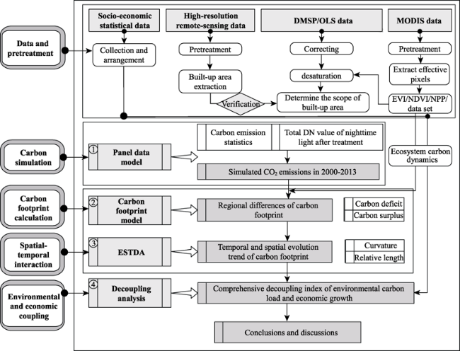
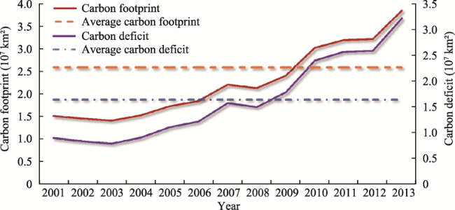
In 2007, China surpassed the USA to become the largest carbon emitter in the world. China has promised a 60%-65% reduction in carbon emissions per unit GDP by 2030, compared to the baseline of 2005. Therefore, it is important to obtain accurate dynamic information on the spatial and temporal patterns of carbon emissions and carbon footprints to support formulating effective national carbon emission reduction policies. This study attempts to build a carbon emission panel data model that simulates carbon emissions in China from 2000-2013 using nighttime lighting data and carbon emission statistics data. By applying the Exploratory Spatial-Temporal Data Analysis (ESTDA) framework, this study conducted an analysis on the spatial patterns and dynamic spatial-temporal interactions of carbon footprints from 2001-2013. The improved Tapio decoupling model was adopted to investigate the levels of coupling or decoupling between the carbon emission load and economic growth in 336 prefecture-level units. The results show that, firstly, high accuracy was achieved by the model in simulating carbon emissions. Secondly, the total carbon footprints and carbon deficits across China increased with average annual growth rates of 4.82% and 5.72%, respectively. The overall carbon footprints and carbon deficits were larger in the North than that in the South. There were extremely significant spatial autocorrelation features in the carbon footprints of prefecture-level units. Thirdly, the relative lengths of the Local Indicators of Spatial Association (LISA) time paths were longer in the North than that in the South, and they increased from the coastal to the central and western regions. Lastly, the overall decoupling index was mainly a weak decoupling type, but the number of cities with this weak decoupling continued to decrease. The unsustainable development trend of China’s economic growth and carbon emission load will continue for some time.

Cite this article

ZHANG Yongnian , PAN Jinghu , ZHANG Yongjiao , XU Jing . Spatial-temporal characteristics and decoupling effects of China’s carbon footprint based on multi-source data[J]. Journal of Geographical Sciences, 2021 , 31(3) : 327 -349 . DOI: 10.1007/s11442-021-1839-7

1 Introduction

Global warming is a serious challenge to human survival and sustainable development on planet Earth. Reducing CO2 and other greenhouse gases (GHG) has become a universal issue. In the past 40 years, anthropogenic GHG emissions have been increasing continuously, with the proportion of CO2 produced by fossil fuel combustion and industrial processes reaching 78% (IPCC, 2013). According to data released by the National Oceanic and Atmospheric Administration of the United States (NOAA), the annual average concentration of CO2 in the global atmosphere exceeded 400 ppm for the first time in 2016, which represents an increase of 18.1%, compared with 338.80 ppm in 1980 (NOAA, 2018). The total global carbon emissions in 2016 reached 33.432 billion tons, corresponding to an increase of 14% over the past 10 years. An important consensus has developed amongst the international community that reducing the emissions of GHGs, such as CO2, and promoting the development of a green circular economy are essential in order to deal with climate change.
Since the implementation of the reform and opening up policy in 1978, China's potential for industrialization and urbanization have been stimulated while maintaining rapid economic growth, which has been the drive for a continuous increase in the demand for energy (Wang and Huang, 2019). According to the BP World Energy Statistics Yearbook (2019), China's CO2 emissions in 2018 increased by 2.5% over the previous year, accounting for 28% of the world's total CO2 emissions. As a comparison, the percentage of China's CO2 emissions in 2005 as a proportion of the world's total emissions was 20.9% (BP, 2019). In confronting the intense international pressure for carbon emission reductions at the Paris Climate Conference in 2015, China promised to reduce CO2 emissions per unit GDP by 60%-65% in 2030, compared with that in 2005, requiring a strong decoupling between economic development, resource consumption, and carbon emissions. It is clearly apparent that China is facing huge challenges in attempting to reduce CO2 emissions while maintaining reasonable economic growth. Due to substantial differences amongst the regions in China, in terms of economic and social development as well as energy consumption structures, accurate, scientific measurements and analysis on the spatial and temporal changes in carbon emissions are the key to formulating carbon emission reduction policies that are appropriate considering the characteristics of the different regions themselves.
Given this background, most current research on carbon emissions is focused on carbon emission measurements (Lu et al., 2013), carbon emissions-related influencing factors (Zhou et al., 2017), the evolution of carbon emissions and economic growth (Zhang et al., 2015), the evolution of carbon emissions and energy structures (Xiao et al., 2019), and carbon emission reduction pathways (Zhou and Wu, 2019), etc. However, research analysis on the sources of carbon emissions is relatively scarce (Wang et al., 2010). A carbon footprint analysis investigates carbon emissions from a life cycle perspective, which can facilitate the formulation of scientifically-based and reasonable carbon emission reduction plans from specific sources. This method has received significant attention from the research community in recent years (Lu et al., 2013; Zhang et al., 2018). At present, although there is no common consensus on the definition of a ‘carbon footprint' in academia, it can be roughly summarized in one of two ways. The first is to define carbon footprint as the carbon emission derived from human activities, namely, from the perspective of the societal system with “carbon weight” as the unit of measurement (Rees, 1992). The second is to view carbon footprint as a part of the ecological footprint—the ecological carrying capacity required to absorb CO2 emission from fossil fuel combustion, that is, from the perspective of the natural-societal system, which is measured by the “carbon area” (Wiedmann et al., 2007).
This study utilized the latter specifically, adopting the definition used by the Global Footprint Network (GFN), “carbon footprint refers to the area of productive land (vegetation) that is required to absorb CO2 (through photosynthesis) emitted by fossil fuel combustion”. Research on carbon footprints covers a wide range of topics and is rich in content. Scholars have focused on the concept connotation (Xiao et al., 2019), calculation methods (Mancini et al., 2016), case studies of carbon footprints (Röös et al., 2013), etc. The calculation methods in these studies can be divided into “bottom-up” methods based on a process analysis and “top-down” methods based on an input-output analysis (Alvarez et al., 2015). The studies cover different scales, such as individuals (Kenny, 2009), families (Steen-Olsen et al., 2016), enterprises (Adewale et al., 2019), industries (Cadarso et al., 2015), cities (Chen et al., 2012), regions (Harris et al., 2012), and countries (Wolfram et al., 2016). In China, most of the carbon footprint research studies are follow-ups to foreign research. Some scholars have measured and analyzed the carbon footprints of isolated individual cases from the perspective of different industries or various regions, such as pastoral areas (Zhao et al., 2010) or urban areas (Zhang and Zhang, 2012). Generally speaking, however, domestic research on carbon footprints is still in its infancy, mainly focusing on individual case studies of single region at the microscale, while research on the mesoscale, macroscale, or on regional differentiation of carbon footprints is relatively lacking. In addition, different scholars use different measurement methods, data acquisition methods, emission source classifications, CO2 emission coefficients, etc. Thus, the calculated results of carbon emissions and carbon footprints are often very different from each other. Because existing research has mainly selected the province as the statistical analysis unit, studies and data at the city level or at smaller scales are severely lacking. Therefore, the research results cannot really be used in a consistent spatial grid of the regions.
Based on the above analysis, identifying “space” and “fine scale” as the goals, this research selected carbon emissions and carbon footprints as its research targets. The pre-processing of basic remote-sensing data from multi-sources, such as DMSP-OLS nighttime lighting data, MODIS NDVI and EVI products, high-resolution remote sensing image data, basic geographic vector data, and economic statistical data, enabled three main parts of this study. First, we established the quantitative relationship between nighttime light values and carbon emission statistics of energy consumption using a panel data model, which was further used to simulate carbon emissions and their spatial distribution in China between 2000 and 2013. Second, we analyzed the spatial-temporal patterns and path evolution characteristics of carbon footprints from the perspective of the natural-societal system by introducing MODIS-NPP products and the Exploratory Spatial-Temporal Data Analysis Method (ESTDA). Third, we interpreted the relationship between urban carbon emission loads and economic growth at the basic unit of prefecture-level cities up to the regional and national level by applying a decoupling theory. The ultimate goal of the third part was to provide decision-making references for the precise implementation of carbon emission reduction targets and “common but different” regional carbon emission reduction policies.

2 Data and research methods

2.1 Data sources and processing

In this study, DMSP-OLS stable nighttime light data from 2000 to 2013 were obtained from the website of the National Centers for Environmental Information (NCEI) of the United States (http://ngdc.noaa.gov/eog/down-load.html). The spatial resolution of this nighttime light data is 30", and the gray value range is 0-63. In this study, based on existing research (Pan and Li, 2016; Zhao et al., 2019), the raw nighttime light data was desaturated using Vegetation Enhanced Index (EVI) data to construct three kinds of indices, namely, the Ratio Nighttime Light Vegetation Index (RVI), Modified Difference Nighttime Light Vegetation Index (MDVI), and Enhanced Nighttime Light Vegetation Index (ENVI). The mutation detection method was used to determine the optimal threshold. Three sample cities, Beijing, Shenzhen, and Xi'an, were selected as targets to determine the optimal threshold value for the segmentation of urban built-up areas, which was calculated using MATLAB software. Due to space limitations, readers can refer to the following publications, which contain the detailed processing procedures: Pan and Li (2016), Zhang and Pan (2019) and Zhuo et al. (2015).
Carbon emission statistics were extracted from the China Emission Accounts and Datasets (CEAD) (http://www.ceads.net/). The database was jointly established and compiled by research institutions in China, Great Britain, the United States, the European Union, and Japan. It includes national, provincial, and urban (partial) energy and carbon emission inventories in long-term series (1997-2015). The inventory database includes carbon emission data from 14 industrial processes and 17 energy generation types.
The Normalized Difference Vegetation Index (NDVI) data (MOD13A2), the EVI data (MOD13A2), and the Net Primary Productivity (NPP) data (MOD17A3) from 2000 to 2013 were obtained from a NASA database (https://search.earthdata.nasa.gov/search). NDVI and EVI data are 16-day composite data with a spatial resolution of 1 km. The monthly data from May to September of each year were selected for mosaic, clipping, and projection conversion as well as other processes. To eliminate the influence of outliers, the annual NDVI and EVI based on compiled monthly data were obtained by the maximum value synthesis method. NPP data are annual data with a spatial resolution of 1 km. Land use data (MCD12Q2) from 2001 to 2013 were obtained from NASA with a spatial resolution of 1 km. Using the first type of International Geosphere Biosphere Programme (IGBP) global vegetation classification scheme, the land covered with vegetation (referred to as the productive land) was extracted from the various land cover types.
The high-resolution remote sensing images were obtained from Google Earth with a spatial resolution of 7 m, which were compared with the nighttime light data from built-up areas to verify the extraction accuracy. The socio-economic statistical indicators were derived from the China Regional Economic Statistical Yearbook (2001-2014) and the China Urban Statistical Yearbook (2001-2014). The Hong Kong and Macao Special Administrative Regions, Taiwan Province, and Tibet Autonomous Region were not included in the analysis due to a lack of data. The administrative boundaries and city locations were obtained from the 1:4,000,000 database of the National Geomatics Center of China, while the standard map production No. GS (2016) 2885 was downloaded from the standard map service website of the Ministry of Natural Resources (http://bzdt.ch.mnr. gov.cn/), and this base map was not modified.

2.2 Research methods

2.2.1 Panel data model
Panel data analysis can utilize the information from samples in two dimensions of different geographic scales and time series to build a multi-dimensional measurement model. Compared with the common regression model, the panel data model allows for increased freedom of data, reduced collinearity problems, and has incomparable advantages in the identification and measurement of dynamic processes and effects. The model expression is (Chen, 2014):
${{y}_{it}}={{\alpha }_{i}}+{{\beta }_{i}}{{x}_{it}}+{{u}_{it}}$
where xit = (x1t, x2t, ..., xnt)T is an independent variable with dimension of 1 × K, αi is a constant term, βi is a coefficient variable with dimension of 1 × K, ${{u}_{it}}$is a random error term of cross section i, and time is t (i = 1, 2, ..., n; t = 1, 2, ..., T).
There are usually three models for panel data analysis: (1) the mixed regression model; (2) the fixed effect model; and (3) the random effect model. When panel data are used for analysis, the specific selection and application of the three different models are mainly determined by the F test. If the F test accepts the original hypothesis, it is considered that the intercept terms and slope coefficients of different individual data models are statistically the same. In that case, the mixed regression model is selected. Otherwise, the fixed effect model or random effect model is selected. The result of the Hausman test is used to screen out the fixed effect model or random effect model. If the Hausman test shows that the individual effect is related to the regression variable, the fixed effect model is selected. Otherwise, the random effect model is selected. There are four main steps in simulation modeling when using panel data: (1) the unit root test; (2) the co-integration test; (3) the selection of the panel data model; and (4) building a panel regression model. Due to space limitations, please refer to Xu et al. (2008) for details on the various inspections, measurements, and statistical formulae.
2.2.2 Research methods on carbon footprints and carbon deficits
In this study, the carbon footprints were calculated from the perspective of the natural ecosystem and the societal economic system. The NPP data were introduced as the carbon absorption index of the ecosystem. Further, the area of productive land (vegetation) was extracted from land cover data products. The carbon footprint measurement model was established as follows (Jiang et al., 2014; Wu et al., 2014):
$C{{F}_{it}}=\frac{C{{T}_{it}}}{NP{{P}_{it}}}\times {{S}_{it}}$
$\Delta C{{F}_{it}}=C{{F}_{it}}-{{S}_{it}}$
where CFit is the carbon footprint (km2) of region i in year t, CTit is the carbon emissions (Pg C/a) from energy consumption in region i in year t, Sit is the productive land area (km2) of region i in year t, and NPPit is the total net primary productivity (Pg C/a) of region i in year t. When the carbon absorption capacity of the regional ecosystem is not enough to absorb the CO2 produced by its energy consumption, the carbon deficit (ΔCFit > 0) is triggered, indicating that the regional economic development and the environment are in an unsustainable state, and vice versa in the case where there is a carbon surplus (ΔCFit < 0).
2.2.3 Exploratory spatial-temporal data analysis (ESTDA)
The analysis of spatial effects has become an effective means of revealing imbalances or convergences of regional development, and can effectively depict the comprehensive processes and patterns of geographical segments. However, the existing empirical research on spatial pattern differences and evolutionary characteristics of geographic variables requires more data points to make cross-sectional representations and to separate spatial and temporal patterns. Thus, the coupling and continuity of spatial and temporal elements are often neglected. However, to utilize the existing framework of the Exploratory Spatial Data Analysis (ESDA), both spatial and temporal factors should be integrated. Rey and Janikas (2006) proposed the ESTDA method by effectively integrating time and space under the traditional ESDA analysis framework. In this study, we applied the ESTDA method to comprehensively analyze the pattern differentiation and evolutionary characteristics of carbon footprints in global and local spaces.
ESTDA is a collection of spatial data analysis methods and technologies. Based on the measurement of spatial-temporal evolutions in spatial correlation, it ascertains spatial agglomeration and spatial differentiation through the description and visualization of temporal dimensions, revealing spatial distribution pattern changes of geographies or activities. The main research methods include Global Moran's I, the LISA index, a scatter plot of LISA, a spatial-temporal transition of LISA, the spatial Markov chain, etc. Moran's I index is used to measure and analyze the spatial characteristics of the carbon footprint of a whole region, and judge whether there is a potential spatial relationship in the distribution of the carbon footprint. The LISA time path is integrated to incorporate the dynamic migration of LISA coordinates in the Moran scatter plots. Through the pairwise movement of the attribute and spatial lag values of the carbon footprint of prefecture-level cities over time, the spatial-temporal interactions and dynamic characteristics of the carbon footprint at the local level within regions are thus explained. Expression of the local spatial dependence from the “instantaneous scene” to the “interactive dynamic scene” is continuously depicted. The geometric characteristics of the LISA time path mainly include relative length (Гi) and curvature (Δi), and their respective expressions are as follows (Gao et al., 2014):
${{\Gamma }_{i}}=\frac{n\times \sum\limits_{\text{t=}1}^{T-1}{d\left( {{L}_{i\text{,}t}}\text{,}{{L}_{i\text{,}t+1}} \right)}}{\sum\limits_{i=1}^{n}{\sum\limits_{\text{t=}1}^{T-1}{d\left( {{L}_{i\text{,}t}}\text{,}{{L}_{i\text{,}t+1}} \right)}}}$
${{\Delta }_{i}}=\frac{\sum\limits_{\text{t=}1}^{T-1}{d\left( {{L}_{i\text{,}t}}\text{,}{{L}_{i\text{,}t+1}} \right)}}{d\left( {{L}_{i\text{,}1}}\text{,}{{L}_{i\text{,}T}} \right)}$
where T is the interval for the time series, n is the number of prefecture-level units, and Li,t is the LISA coordinate position (carbon footprint standardization value, carbon footprint space lag) of prefecture-level unit i in year t. In other words, (yi,t,yLi,t). d (Li,t,Li,t+1) is the coordinate for the distance moved by prefecture-level unit i in year t to t+1. If the length of the coordinate movement of prefecture-level unit i is greater than the national average in the studied time range, then the city's Γi is greater than 1. The larger the Γi value, the more dynamic the local spatial dependence and spatial structure of the carbon footprint for prefecture-level unit i, and vice versa. The larger the ∆i, the more curved the LISA time path; namely, it is more affected by neighborhood space (spillover/polarization) in city i, and city i has a more volatile carbon footprint process and spatial dependent evolutionary process. In the opposite situation, the impact is less. The spatial-temporal transition of LISA reflects the transformation process of local spatial association types in the studied time range. There are four types of spatial-temporal transitions. Type I is the diagonal type of transfer matrix, which means that there is neither spatial transfer within the prefecture-level unit itself nor between the neighboring cities. Type II refers to a transition within the prefecture-level unit itself, but the neighborhood is unchanged. Type III refers to no change within the prefecture-level unit itself, but its neighborhood has a transition. Type IV refers to a transition within the prefecture-level unit and in its neighborhood. From the known transition types, the spatial stability of Moran's I can be calculated with the following expression (Gao et al., 2014):
${{S}_{t}}=\frac{{{F}_{0,t}}}{n}$
where F0,t represents the number of prefecture-level units where the transition of Type 0 has occurred in the time range of t, while n is the number of prefecture-level units where all transitions may occur.
2.2.4 Analysis of decoupling effects
The term “decoupling” is derived from physics and refers to the interruption and disconnection of the relationship between two or more physical quantities. It was introduced into the field of economics to study the coupling relationship between economic growth and resource consumption or environmental pollution and reflect the sensitivity of resource and environmental pressure changes to economic changes. At present, most research find an elastic relationship between carbon emission growth and GDP growth within a specific time period. In this study, carbon emissions and carbon footprint pressure indicators were introduced to measure the elasticity of economic growth, in which GDP represents the economic variable. Considering the differences in regional carbon absorption capacities, the “carbon footprint pressure” variable was introduced and is defined as the ratio of total carbon emissions from the energy consumption of the regional economy to the regional terrestrial carbon absorption capacity. It can more completely and synthetically measure the coupling or decoupling relationship and degree of influence between human economic activities, resources, and the environment. Based on the Tapio decoupling model, the following decoupling model was constructed (Wang and Li, 2015):
$CB{{I}_{it}}=\frac{C{{T}_{it}}}{NP{{P}_{it}}}$
$e=\frac{\left( \Delta \text{C}{{\text{O}}_{\text{2}}}/\text{C}{{\text{O}}_{\text{2}}}+\Delta CBI/CBI \right)/2}{\Delta \text{GDP}/\text{GDP}}$
where CBIit is the carbon footprint pressure index of region i in year t; CTit is the total carbon emission generated by the energy consumption of region i in year t; NPPit is the carbon absorption capacity of region i in year t; e is the decoupling elasticity; ∆CO2, ∆CBI, and ∆GDP represent the growth of carbon emissions, carbon footprint pressure, and GDP, respectively, between the start and end years of the studied time period. According to the value of the elasticity, the decoupling states have been classified into the following eight types: strong decoupling, weak decoupling, weak negative decoupling, strong negative decoupling, expansion negative decoupling, expansion connection, recessive decoupling and recessive connection. See the literature for the specific classification standard (Wu et al., 2013; Zhong et al., 2010).
Figure 1 The analysis framework for spatial-temporal patterns in carbon footprints and the decoupling levels

3 Results

3.1 Spatial and temporal distribution of carbon emissions

Based on sample data from provinces in the central region, the model and its parameters were established with the panel data model method at a grid scale by correlating the sample data from selected areas to their nighttime light image data (after systematic correction) to simulate nationwide carbon emissions. The LL test (same root) and IPS test (different root) were applied to evaluate the stationarity of the panel data. A natural logarithm transformation was performed on all data to avoid heteroscedasticity and non-stationary phenomena. The test results showed that, at the 1% significance level, all probabilistic values and test statistics, including the panel PP-Statistic, panel ADF-Statistic, group PP-Statistic, and group ADF-Statistic, supported the idea that a long-term equilibrium and co-integration equation between LnNTL and LnTCO2 existed. Since the residual of the regression equation was stationary, the panel regression equation was performed. Thus, the F-test and Hausman test could be used to screen out the models. The results showed that the F-test rejected the original hypothesis. Using the variable coefficient model, the P value of the Hausman test was 0.421, which implied that the random effect model was more reasonable than the fixed effect model. The random effect model was then established based on the statistical value of the total nighttime light data in the built-up areas and the CO2 emissions of the corresponding cities. The P value was 0, indicating that there was significant correlation at the 1% significance level with an R2 value of 0.874. The model structure is described as follows:
$\text{ln}T\text{C}{{\text{O}}_{\text{2}}}=0.36\text{ln}NTL+2.73$
The simulated spatial distribution of carbon emissions in China from 2000 to 2013 is shown in Figure 2. The carbon emission statistics of both provincial units, such as Beijing, Qinghai, and Xinjiang, and prefecture-level cities, such as Changsha, Fuzhou, Kunming, and Shangrao (a total of 28 validation samples), were used to verify the accuracy of the simulation results in 2002, 2007, and 2012. It was found that the simulated values reflected the statistical distribution of carbon emissions closely, and that there was an obvious linear relationship between these two datasets. Accordingly, the coefficient of determination R2 for the three selected periods was 0.893, 0.955, and 0.951, respectively.
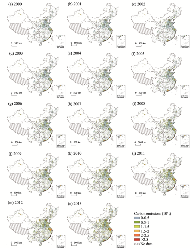
Figure 2 Spatial distribution of carbon emissions in China from 2000 to 2013

3.2 Spatial patterns of carbon footprints

This study attempted to determine carbon footprints from the perspective of the natural-societal system to analyze the ecological capacity required to absorb the CO2 released from fossil fuel combustion in the corresponding geographic area. The carbon dioxide absorption capacity of the natural ecosystem has regional differences. When the carbon emissions exceed the maximum absorption capacity of the local natural ecosystem, it is referred to as a carbon deficit, indicating that the natural-societal system is in a state of unsustainable development.
3.2.1 National scale
Figure 3 shows increasing trends for both carbon footprint and carbon deficit in China from 2001 to 2013. In 2001, China's carbon footprint was 1.476 × 10⁷ km2, while the productive area of the land system was 0.613 × 10⁷ km2, resulting in a carbon deficit area of 0.863 × 10⁷ km2. In 2013, China's carbon footprint was 3.808 × 10⁷ km2, and the carbon deficit area reached 3.181 × 10⁷ km2. The annual growth rates of the carbon footprint and carbon deficit were 4.82% and 5.72%, respectively. Since 2008, the growth rates of both the carbon footprint and carbon deficit have been increasing more conspicuously than in the preceding periods.
Figure 3 Variation trends of the carbon footprint and carbon deficit in China from 2000 to 2013
3.2.2 Provincial scale
The calculated results of China's carbon footprint were classified into five categories based on the standard deviation classification method and are shown in Figure 4. In 2001, regions with larger carbon footprints were mainly located in the North China Plain, Shandong Peninsula, and Guangdong Province. Among them, the Shandong Province possessed the largest carbon footprint (145 × 104 km2). Regions with smaller carbon footprints were located in the hilly areas of the southwest and south of China. Among them, Hainan Province possessed the smallest carbon footprint (3.53 × 10⁴ km2). By 2007, the locations of regions with large carbon footprints had gradually moved to the northeast with Inner Mongolia becoming the province with the largest carbon footprint (225 × 104 km2). Meanwhile, the carbon footprint of Xinjiang showed significant growth. By 2013, Inner Mongolia and Xinjiang had become the “burgeoning” growth areas in terms of carbon footprint. The sum of the carbon footprints of these two regions combined was 860 × 104 km2, indicating intense regional differences and imbalances. The provinces with the highest annual growth rate in their carbon footprint were Qinghai Province (5.65%), followed by Inner Mongolia (5.62%), and Xinjiang (5.60%). The central and western regions of China also had high growth rates. In regions like Tianjin, Shanxi and Hebei provinces with high energy consumption and high carbon emissions, the carbon footprints were, in contrast, growing at a low rate.
Figure 4 Trends in carbon footprint at the provincial level from 2001 to 2013
The ecological supplying capacity (productive land) differs between different provinces and regions of China, which directly affects the potential for carbon absorption in the terrestrial ecosystem. The differences in carbon deficit among the provinces are the result of both human activities and regional ecological supplying capacity. From 2001 to 2013, the changes in carbon deficit/surplus between provinces and regions were significant (Figure 5). In 2001, eight provinces (Chongqing, Jiangxi, Hunan, Guangxi, Guizhou, Yunnan, Sichuan, and Qinghai) held the status of ecological surplus. All these provinces are located in the central and western regions, and the regional ecological carrying capacity is strong, in other words, they could effectively absorb their corresponding carbon emissions. Carbon deficits occurred mainly in areas with industrial or capital-intensive urban agglomeration, such as Beijing, Tianjin, Hebei, Central Plains, Pearl River Delta, and the Yangtze River Delta. By 2007, the number of provinces with a carbon surplus had decreased from eight to four, namely Guizhou, Yunnan, Sichuan, and Qinghai. Among them, Qinghai had the highest carbon surplus (29.5 × 10⁴ km2). Shandong remained the province with the largest carbon deficit, reaching 174 × 104 km2, followed by Hebei and Inner Mongolia. By 2013, all provinces exhibited carbon deficits, with carbon deficits appearing in Qinghai and Yunnan for the first time. Inner Mongolia surpassed Shandong to become the province with the largest carbon deficit (363 × 104 km2), and the central and western regions became the main locations with increasing carbon deficits.
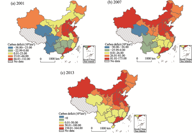
Figure 5 Trends in carbon deficit at the provincial level from 2001 to 2013
3.2.3 Prefecture-level city scale
At different jurisdictional scales, the spatial distribution patterns in carbon footprints and carbon deficits can be inconsistent because of scaling and zoning effects. Prefecture and prefecture-level cities (hereinafter referred to as prefecture-level units) are the backbone of China's administrative system and are the centers of regional economic development. Therefore, research and analysis of carbon footprints and carbon deficits at the prefecture level in China can assist in distinguishing between development patterns and trends at different scales in different regions. To some extent, these can serve as inputs for more precise targeting of carbon emission reductions. In this study, carbon footprints and carbon deficits were calculated for prefecture-level units in 2001 and 2013. The calculated results were classified into five categories according to the standard deviation classification method.
Generally, as shown in Figure 6, the carbon footprints of all prefecture-level units had a wide range in 2001, and showed an obvious pattern of spatial agglomeration. The average carbon footprint of the 336 prefectural units in China was 4.39 × 10⁴ km2 with a standard deviation of 6.06 × 10⁴ km2. The 99 national level cities with higher carbon footprints than the average were mainly distributed in areas north of the Qinling Mountains-Huaihe River. There were 123 cities with low carbon footprints, 149 cities with moderate-low carbon footprints, 40 cities with medium carbon footprints, 17 cities with moderate-high carbon footprints, and 7 cities with high carbon footprints. In 2013, the average carbon footprint of prefecture-level units had almost tripled to 11.33 × 10⁴ km2 with a standard deviation of 13.56 × 10⁴ km2. The number of cities with carbon footprints exceeding the average level of all studied prefecture-level cities had increased by 12, compared with that in 2001, and the central and western regions were the main locations showing increasing carbon footprints. There were 132 cities with low carbon footprints, 137 cities with moderate-low levels, 48 cities with medium levels, 7 cities with moderate-high levels, and 13 cities with high levels. The number of cities with increasing carbon footprints was significant, shifting from the central regions to the western regions.
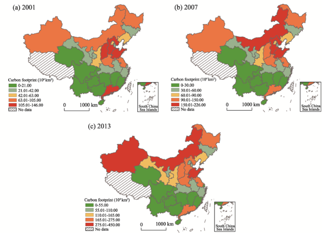
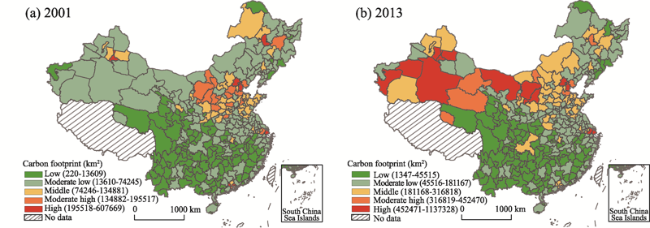
Figure 6 Differentiation patterns of carbon footprints in prefecture-level cities in 2001 and 2013
The calculated carbon deficits were divided into five categories according to the standard deviation method (Figure 7), using 0 as the dividing benchmark between negative values as carbon deficits and positive values as carbon surpluses. As is apparent from Figure 7, the carbon deficits/surpluses of prefecture-level units also showed distinct spatial differentiation and agglomeration. Of the 336 prefectural units in 2001, there were 121 cities with carbon surpluses. Some cities had relatively large carbon surpluses, including the Yushu Tibetan Autonomous Prefecture, Hulun Buir City, Xilin Gol League, Garze Tibetan Autonomous Prefecture, Aba Tibetan and Qiang Autonomous Prefecture. In addition, there were 215 cities with carbon deficits. Among them, capital-technology intensive cities, such as Beijing, Tianjin, and Shanghai, and industrial energy-consuming cities, such as Baotou City, Zhangzhou City, and Handan City, had much larger carbon deficits.
By 2013, the carbon deficit and carbon surplus of each prefecture-level city had changed significantly. The number of cities with carbon surpluses had decreased sharply, and the spatial distribution of these cities had moved rapidly to the west. In contrast, the cities with carbon deficits had gradually spread out to the northwest, and areas with relatively high carbon deficits mainly concentrated on the northern and southern sides of 35°N. The number of prefecture-level units with carbon surpluses decreased from 121 to 31, while conversely the number of prefecture-level units with carbon deficits increased to 305.
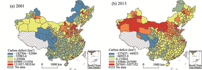
Figure 7 Differentiation patterns of carbon deficits and carbon surpluses in prefecture-level cities in 2001 and 2013

3.3 Spatial and temporal evolution trends in carbon footprints

3.3.1 Evolutionary trend of overall pattern
The coefficient of variation (CV) and global Moran's I index for each prefecture-level unit were calculated to comprehensively analyze the characteristics of the evolutionary trends in the spatial-temporal patterns in the carbon footprints from 2001 to 2013. The CV showed a “wave-like” trend at first with an increase, then a decrease followed by another slow increase before reaching its lowest value of 0.789 in 2003. Thereafter, the CV increased year after year to a maximum of 0.861 in 2013.
The global Moran's I index of each prefecture-level unit was calculated using GeoDa software. The value of the Z statistic was greater than 2.58 at the 1% significance level, and the global Moran's I index maintained at 0.491 for many years, indicating that there was significant spatial autocorrelation of the carbon footprints at the prefecture level. Thus, cities with higher carbon footprints were spatially agglomerated, and the surrounding cities also had relatively high carbon footprints. After a growth of the global Moran's I index to 0.465 in 2002, it dropped to 0.433 in 2003, and then gradually increased to 0.544 in 2013. This reflects the progressively increasing spatially agglomeration of the carbon footprints of prefectural units over time.
3.3.2 Evolutionary trends in local spatial patterns
(1) Relative lengths of LISA time paths
From the perspective of spatial and temporal dimensions, the relative length of LISA time paths can reveal the influence of local activity on the stability of the spatial structure. In this study, based on the natural breakpoint method coupled with manual classification (dividing a critical value greater than 1, that is, greater than the national average), the relative lengths of the LISA time paths were divided into seven classes. From Figure 8, it is apparent that the relative lengths of the LISA time paths were longer in the North than that in the South, and it increased from the coastal areas to the central and western regions. This indicates that the local spatial structure of the carbon footprints in the central and western regions was more dynamic, while it was more stable in the southwest and southeast regions.
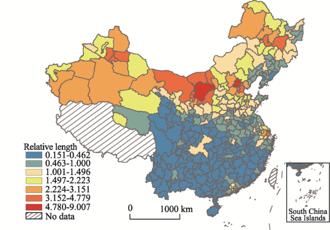
Figure 8 The relative length of LISA time paths of China's carbon footprints from 2001 to 2013
The LISA time paths with relatively long lengths were found principally in Beijing-Tianjin-Hebei, the core cities of the Yangtze River Delta, as well as the northern slopes of the Tianshan Mountains, Hohhot-Baotou-Ordos-Yulin Area, and Songnen Plain. The relative length of the LISA time path for each capital city ranked top in its own province. Among the 30 capital cities or municipalities, the average relative length of the LISA time path was 1.831. Of these cities, 66.7% had LISA time paths whose relative lengths were greater than 1. Among the 336 prefecture-level units, there were 113 with LISA time paths whose relative lengths were greater than 1. Furthermore, the relative length of the LISA time paths exceeded 3.5 in cities such as Beijing, Wuhai, and Alashan, while for cities such as Liangshan, Panzhihua, and Hechi, the relative lengths of the LISA time paths were below 0.19. Such differences in the stability of the spatial structure can provide an instructive direction for emissions reduction targets with a focus on prevention and optimization. Regions with more dynamic interactions in their spatial structures need to devote greater efforts to reform and accelerate the elimination of industries with poor productivity as part of the process of industrial development, as well as facilitate the operation and promotion of a low-carbon economy. Regions with relatively stable spatial structures should further facilitate the innovations and upgrades to low-carbon technologies, broaden the applications of clean energy in industrial production and residential use, and enhance the carbon absorption capacity of the ecological environment to reduce their carbon deficit.
(2) Curvature of LISA time paths
The curvatures of the LISA time paths were divided into seven classes. The greater the value of the curvature, the larger the effect on the carbon footprint of the neighboring space (spillover/polarization), while the spatial dependence also had great volatility. As shown in Figure 9, the curvatures of the LISA time paths show a decreasing trend from the coastal areas to the inland areas, and this distribution pattern is roughly opposite to the relative lengths of the LISA time paths. The mean curvature values of the time paths showed a decreasing trend in these areas: northeast (9.89) > central (8.05) > eastern (7.09) > western (4.03). From a regional scale, regions with high curvatures in their carbon footprints were mainly located in the Greater and Lesser Khingan mountains; northeastern, central and eastern parts of China such as Huaibei, Wuhan, and southern Hunan; southeastern coastal areas and the Leizhou Peninsula, reflecting large fluctuations in the spatial influence in these areas. Regions with low curvatures in their carbon footprints were mainly concentrated in the northwest, Central Plains, North China, Pearl River Delta, and Southwest China, indicating a relatively stable spatial relationship in these regions. The average curvature value among the 336 prefecture-level units was 6.231 with a standard deviation of 8.544. Out of the 336 prefecture-level units, curvature values greater than the national average value were shared by 106 units. Among them, 11 cities possessed curvature values greater than 18, including Hengyang, Hangzhou, and Shaoxing. The curvature values in 10 cities, including Jiayuguan, Jiuquan, and Zhangye, were less than 2. These cities had higher carbon footprint growth similar to their neighboring cities, such that the fluctuations in the spatial relationships were mutually restrained, resulting in smaller curvature values.
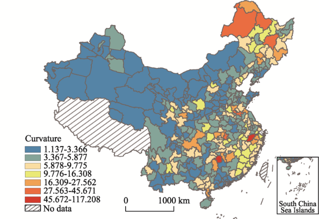
Figure 9 Tortuosity of the LISA time paths of China's carbon footprints from 2001 to 2013
(3) Spatial-temporal transitions of LISA
While the LISA time paths revealed the dynamic migration trend in the LISA coordinates of carbon footprints of different prefecture-level units in the Moran scatter plot, the spatial-temporal transitions of LISA can reveal the characteristics of a transfer in local spatial correlation types for carbon footprints. As can be seen in Table 1, the spatial correlation pattern remained relatively stable for the prefecture-level units. The spatial stability of the carbon footprints in Moran's I was 0.933, which indicates that the probability of no spatial-temporal transition in local spatial correlation for each prefecture-level unit over the 14 years was 93.3%. This reflects the strong stabilizing characteristics of the prefecture-level units.
Table 1 Spatial-temporal transition matrix of carbon footprints of prefecture-level units in China
t/t+1 HH (Deep
pressure type)
LH (Sunken type) LL (Weak
pressure type)
HL (Polarization
type)
HH (Deep pressure type) Type 0 (0.251) Type I (0.007) Type III (0.002) Type II (0.002)
LH (Sunken type) Type I (0.009) Type 0 (0.121) Type II (0.013) Type III (0.000)
LL (Weak pressure type) Type III (0.003) Type II (0.019) Type 0 (0.514) Type I (0.005)
HL (Polarization type) Type II (0.004) Type III (0.000) Type I (0.003) Type 0 (0.047)
The high to low probability of the four types of spatial-temporal transitions occurring were: Type I (0.933) > Type III (0.038) > Type II (0.024) > Type IV (0.005), which shows that the dominant position was no spatial association transfer. The spatial associations showed transitional inertia to varying degrees. For Type III, activities of spatial-temporal transition in surrounding areas were more pronounced, while the central units themselves were relatively stable. The lowest probability of spatial-temporal transition was Type IV, which means that the spatial correlation transfer within the city itself and its surrounding cities was relatively rare. The most common spatial correlation transition in Type I was LL (Low-Low) → LL (probability of 0.514). For Type II, the highest transition probability of spatial correlation was LH (Low-High) → HH (High-High) (0.009), reflecting the transformation of the spatial correlation of the carbon footprint for prefecture-level cities from “sunken type” to “deep pressure type.” Some low-carbon footprint cities were affected by the surrounding cities, as the size of carbon footprints continued to increase. The least likely spatial correlation transition was HL (High-Low) → LL (0.003), as the probability of transferring from high-carbon footprint cities to low-carbon footprint cities was very small, showing that economic prosperity was still driven by high energy consumption in most cities, which were relatively lacking in investment in green and low-carbon economic system reforms. For Type III, the highest probability of spatial correlation transition was LH (Low-High) → LL (0.033), indicating that the influence from neighbors' carbon footprints in some areas experienced a partial relief. However, its probability was still lower than that of other types. The lowest probability of spatial correlation transition was HH → HL (0.003). For Type IV, the highest probability of spatial correlation transition was LL → HH (0.033) and the lowest were LH → HL (0.000) and HL → LH (0.000).

3.4 Results and analysis of calculated comprehensive decoupling index

Using the improved Tapio decoupling formula, a comprehensive decoupling index of the carbon emission load and economic growth in 336 prefecture-level units were calculated. The elastic characteristics of the carbon emission load relative to economic growth in the prefecture units starting in 2001 were analyzed. It was noteworthy that there were no units with GDP < 0 in the studied period, and therefore, there were only four kinds of decoupling: strong negative decoupling, weak negative decoupling, receding decoupling, and expanding connection. Because of the hysteretic characteristics of economic growth, changes in energy consumption and carbon cycle absorption over a multi-year period need to be used to analyze any decoupling (Wu et al., 2010). Therefore, in this study, the analysis was done using a comprehensive decoupling index to identify a decoupling status for each unit over the three time periods, 2001-2005, 2005-2009, and 2009-2013 (Figure 10).
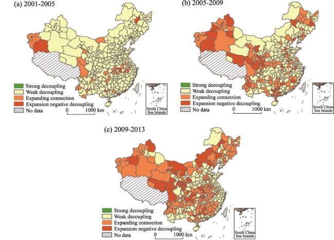
Figure 10 Spatial patterns of the carbon emissions load decoupling levels in China from 2000 to 2013
As shown in Figure 10, the decoupling of the carbon emission load from economic growth changed significantly over the three periods. Overall, the main types of decoupling that occurred in the three periods were weak decoupling, expanding connection, and expanding negative decoupling. The number of areas with an expanding connection and an expanding negative decoupling increased gradually and these areas shifted to the central, western, and northeastern regions. Specifically, from 2001 to 2005 (first phase), the main type of decoupling was weak decoupling exhibited by 304 cities. A total of 25 cities typified an expanding connection type, while 4 cities typified an expanding negative decoupling type. Only Hebei and Jinzhou typified a strong decoupling type. The national average decoupling elasticity value was 0.396 with a CV of 1.214. From 2005 to 2009 (second phase), the category of expanding connections expanded significantly from 25 to 84 cities in the second phase. The number of weak decoupling cities decreased by 87, while the number of negative decoupling cities increased by 31, showing that the changes were mainly caused by the influence of urban neighbors on their surrounding areas in the northwest, and from expansion of cities along the north and south sides of the middle and upper reaches of the Yangtze River. The national average elasticity value was 0.795 with a CV of 0.984. The average decoupling value increased, while the CV declined, indicating that the negative external impacts of human economic activity on the environment increased. Also, the degree of difference in the decoupling index between prefecture-level units gradually narrowed. From 2009 to 2013 (third phase), the number of expanding connection cities increased by 9.8%, a continuation of the same phenomenon seen in the second phase. Expanding connection and expanding negative decoupling were mainly exhibited in the northwest and northeast regions and in the hinterland of the upper and middle reaches of the Yangtze River, displaying an “E”-shaped distribution pattern from north to south. As compared with the second phase, the average elasticity value increased by 0.027 and the CV decreased by 0.497.
Figure 11 shows the number of prefecture-level units that changed decoupling types from one period to another. From the trends of decoupling statuses, it is apparent that there were 230 prefecture-level units that did not undergo changes between the first and second phases. Among them, 225 units exhibited weak decoupling, which was the most common type of decoupling, and remained stable during this period. There were 106 prefecture-level units that did change, of which 32 cities went from weak decoupling to an expanding connection type, 17 cities went from weak decoupling to expansion negative decoupling, and 21 cities went from expansion connection to weak decoupling. In the second and third phases, there were 197 prefecture-level units with no decoupling changes. Among those that changed, the number of cities with weak decoupling types had decreased the most by 41 cities. Among the 163 prefecture-level units that had changed, 84 cities had changed from weak decoupling to expanding connection, 24 cities had changed from weak decoupling to expansion negative decoupling, 10 cities had changed from expansion connection to weak decoupling, 6 cities had changed from expansion connection to expansion negative decoupling, and 13 cities had changed from expansion negative decoupling to expansion connection. In general, the weak decoupling state was the most common type of relationship between China's economic growth and carbon emissions. However, it cannot be ignored that the transformation from weak decoupling to expansion connection and expansion negative decoupling continued to increase, while the number of areas with strong decoupling were few. The trend of unsustainable development in China's economic growth and carbon emissions will continue for a certain period of time in the future. This trend means that even more stringent requirements will be needed to reach sustainability in China's economic growth and protection of the environment, which will result in a significant economic transition period.
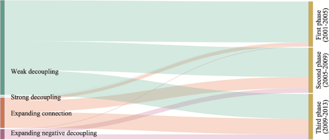
Figure 11 Changes in different decoupling types in prefecture-level cities over three time periods

4 Discussion and conclusions

4.1 Discussion

Seeking the optimal path to carbon emissions reductions on different time and space scales is the key to achieving the short-term, medium-term, and long-term goals of China's green low-carbon transformation while continuing to encourage economic development. Spatial differences at a small scale are more sensitive to macroeconomic fluctuations. The national task of achieving China's carbon emissions reduction goals must be differentiated for the different regions (Zhao et al., 2017). Therefore, it is essential to know how to appropriately divide the regions, identify the key areas, and then implement targeted policies. However, current research is clearly insufficient to delineate the spatial and temporal patterns of China's carbon emissions and carbon footprints. This study found that in 2001, eight provinces and cities (Chongqing, Jiangxi, Hunan, Guangxi, Guizhou, Yunnan, Sichuan, and Qinghai) had carbon surpluses. However, by 2007, the number of provinces with carbon surpluses had decreased to only four, being Guizhou, Yunnan, Sichuan, and Qinghai. In 2013, all the provinces and regions in China held a carbon deficit status. From 2001 to 2013, both carbon footprints and the corresponding carbon deficits were increasing on a yearly basis. The increase in carbon footprints has led to new pressures and presents huge challenges for China's development. With a commitment to ensure social and economic development, we must promote improvements in energy efficiency from the standpoint of policy, the economy, and other aspects, as well as the optimization and adjustment of industrial structures and energy consumption structures. For example, the carbon footprint for cities in central and western China, such as Inner Mongolia and Xinjiang, with energy-rich and chemical-heavy industrial bases, was large and has been rapidly growing. However, considering that the carbon emissions in these areas have been largely due to the provision of high carbon products for the economically developed coastal areas, regional differentiation in terms of emissions reduction responsibilities must account for these factors pertaining to the spatial transfer of carbon emissions.
This study found that there was a significant positive spatial autocorrelation pattern in China's regional carbon footprint, meaning the trend in a region's carbon footprint was affected by the carbon footprint of its neighboring regions. This degree of correlation will continue to increase, and it should be considered during future carbon emissions-related policy-making. Regional cooperation should be strengthened for carbon emission reductions on the macro to micro levels and for regions to enterprises to individuals in order to achieve “precise implementation of emissions reduction measures and precise emissions reductions.” In addition, regional carbon footprints exhibited characteristics of “agglomeration” and “differentiation,” which co-exist within the broader spatial-temporal trends. To achieve the goals of carbon emission intensity reductions to which China is internationally committed, it is necessary to strengthen the monitoring and governance of carbon emission intensity in several key regions and increase constraints on carbon emissions.
Compared with the carbon emission results obtained from the statistical yearbook data through conversions, the CEAD database used in this study has the advantages of comprehensive coverage, a long time span, unified statistical quality, strong comparability, and detailed data; moreover, it is widely used by both domestic and foreign scholars (Shan et al., 2016; Zhu et al., 2019). These data were used as an explanatory variable in this study, combined with the nighttime lighting data to build a panel regression model to depict the spatialization of carbon emissions. However, there was a problem with the DMSP-OLS nighttime data, in that the pixel values were not uniform throughout the continuous time series. Therefore, in this study, the nighttime light data within a given year were integrated and data had to be rectified across different years. Limited by the radiation resolution of the sensor, there were a lot of saturated pixels in the apparent urban centers, which caused the actual differences in light brightness in urban center areas to be masked and regional differences to be homogenized.
There are many studies that have proven a negative spatial correlation between the DN value of nighttime light and the vegetation index value of the corresponding region. In this study, three indices were constructed using EVI data to desaturate the original nighttime light data. The consumption of traditional fossil energy is the main source of GHG emissions and is usually concentrated in urban areas. Therefore, high-precision extraction of urban built-up areas based on nighttime lighting images is the basis of the carbon emission simulation. In this study, the mutation detection method was used to determine the optimal threshold for the segmentation of built-up areas. Thus, high-precision urban built-up area information was extracted, guaranteeing the reliability of the simulation results. By building the panel data model, the quantitative simulation of carbon emissions for a long time series was objectively and systematically realized. Compared with the traditional cross-section data model, the panel data model comprehensively utilizes the sample information and analyze differences between individuals. It can also describe characteristics that have dynamic variation between individuals. Therefore, the results have high test accuracy. Using the improved Tapio decoupling model and ESTDA method, this study delivered insights that expand our current understanding of the spatial-temporal evolution of carbon footprint patterns across China and the decoupling relationship between urban carbon emissions loads and economic growth at the prefecture level. It can also be utilized as a critical reference for formulating “common but different” carbon emissions reduction and control policies.
Although this study used commonly recognized statistical carbon emissions data from CEAD, which are calculated from 17 types of fossil fuel consumption, and are more comprehensive than the statistical data currently generally used by the academic community to estimate carbon emissions, actual carbon emission sources include not only industrial production, but also agriculture, land use, etc., which this dataset omits. Due to the difficulties of data acquisition and statistics, the results obtained through indirect calculations inevitably had some errors when compared with the reality. In addition, the spatial resolution of the DMSP-OLS data was low, and the data were not updated after 2014. The data from the new generation NPP-VIIRS and the domestic Luojia-1 satellite, which adopted on-board radiometric calibration, have improved temporal and spatial resolutions. Using these data to estimate carbon emissions will be the focus of our next research project in order to achieve a continuous time series for carbon emission monitoring and analysis. The processes of carbon emissions and carbon footprints represent very complicated natural-societal systems, and the driving mechanisms are complex. Combined with data on actual societal and economic developments and regional spatial differences in China, identifying more reasonable, actionable, and precise driving mechanisms, through quantitative analysis at small and medium scales, will also be the focus of future research.

4.2 Conclusions

By using DMSP-OLS nighttime lighting data and carbon emission statistics, a panel data model was constructed in this study to simulate China's carbon emissions from 2000 to 2013. Applying the framework of the Exploratory Spatial-temporal Data Analysis (ESTDA) system, this study also analyzed the dynamic evolution of spatial patterns in carbon footprints from 2001-2013. The coupling or decoupling of the carbon emission load and economic growth in 336 prefecture-level units over three time periods (2001-2013) was analyzed using the improved Tapio decoupling model. The conclusions are as follows:
(1) From 2001 to 2013, China's carbon footprint and carbon deficit increased every year. The average annual growth rate of the carbon footprint was 4.82%, and the average annual growth rate of the carbon deficit was 5.72%. The overall carbon footprint and carbon deficit in the North was higher than that in the South. The spatial heterogeneities of the carbon footprint and carbon deficit were obvious when observing different jurisdictional scales.
(2) From 2001 to 2013, the CV of the carbon footprint increased, and the annual average value of global Moran's I index of the carbon footprints for the prefecture-level units was 0.491, which is characteristic of significant spatial autocorrelation. The relative lengths of the LISA time paths were longer in the North than in the South, and they increased from the coastal to the central and western regions. While the curvatures of the LISA time paths decreased from the coast to the inland areas, they were higher in the northeast and central regions, and lower in the East and the West.
(3) The comprehensive decoupling index was dominated by the weak decoupling type, but the number of cities with weak decoupling continually decreased. The number of cities with expansion connection and expansion negative decoupling gradually increased, and these cities were mainly located in the northeast, central and western regions. Overall, the types of decoupling changed dramatically during the studied time period.
[1]
Adewale C, Reganold J P, Higgins S et al., 2019. Agricultural carbon footprint is farm specific: Case study of two organic farms. Journal of Cleaner Production, 229:795-805.

[2]
Alvarez S, Sosa M, Rubio A, 2015. Product and corporate carbon footprint using the compound method based on financial accounts. The case of Osorio wind farms. Applied Energy, 139:196-204.

[3]
BP plc, 2019. The BP statistical review of world energy published in 2019 (2019-06-20). London: British Petroleum (BP), https://www.bp.com/en/global/corporate/energy-economics/statistical-review-of-world-energy.html.

[4]
Cadarso M, Cadarso M, Gómez N et al., 2015. Quantifying Spanish tourism’s carbon footprint: The contributions of residents and visitors: A longitudinal study. Journal of Industrial Ecology, 23(6):922-946.

[5]
Chen Q, 2014. Advanced Econometrics and Stata Applications. Beijing: Higher Education Press. (in Chinese)

[6]
Chen S, Chen B, 2012. Network environ perspective for urban metabolism and carbon emissions: A case study of Vienna, Austria. Environmental Science & Technology, 46(8):4498-4506.

PMID

[7]
Gao C C, Liu X Z, Li M K et al., 2014. Spatiotemporal dynamics of carbon emissions by energy consumption in China from 1995 to 2014. Progress in Geography, 35(6):747-757. (in Chinese)

[8]
Guan D, Shan Y, Liu Z, 2016. CO2 emissions from China’s lime industry. Applied Energy, 166:245-252.

DOI

[9]
Harris N L, Brown S, Hagen S C et al., 2012. Baseline map of carbon emissions from deforestation in tropical regions. Science, 336(6088):1573-1576.

PMID

[10]
IPCC, 2013. The physical science basis. In: Contribution of Working Group I to the Fifth Assessment Report of the Intergovernmental Panel on Climate Change. Cambridge and New York: Cambridge University Press.

[11]
Jiang J L, Xu J G, Wu W J et al., 2014. Patterns and dynamics of China’s human-nature carbon source-sink system. Journal of Natural Resources, 29(5):757-768. (in Chinese)

[12]
Kenny T, Gray N F, 2009. A preliminary survey of household and personal carbon dioxide emissions in Ireland. Environment International, 35(2):259-272.

PMID

[13]
Lu J Y, Huang X J, Cheng Y et al., 2013. Spatiotemporal changes of carbon footprint based on energy consumption in China. Geographical Research, 32(2):326-336. (in Chinese)

[14]
Lu W, Chen C, Su M et al., 2013. Urban energy consumption and related carbon emission estimation: A study at the sector scale. Frontiers of Earth Science, 7(4):480-486.

DOI

[15]
Mancini M S, Galli A, Niccolucci V et al., 2016. Ecological footprint: Refining the carbon footprint calculation. Ecological Indicators, 61:390-403.

DOI

[16]
NOAA, 2018. Global greenhouse gas reference network (2018-05-29). Boulder, CO, USA: National Oceanic & Atmospheric Administration (NOAA), https://www.esrl.noaa.gov/gmd/ccgg/trends/global.html.

[17]
Pan J H, Li J F, 2016. Estimate and spatio-temporal dynamics of electricity consumption in China based on DMSP/OLS images. Geographical Research, 35(4):627-638. (in Chinese)

[18]
Rees W E, 1992. Ecological footprints and appropriated carrying capacity: What urban economics leaves out. Environment and Urbanization, 4(2):121-130.

[19]
Rey S J, Janikas M V, 2006. STARS: Space-time analysis of regional systems. Geographical Analysis, 38(1):67-86.

[20]
Röös E, Karlsson H, 2013. Effect of eating seasonal on the carbon footprint of Swedish vegetable consumption. Journal of Cleaner Production, 59:63-72.

[21]
Steen-Olsen K, Wood R, Hertwich E G, 2016. The carbon footprint of Norwegian household consumption 1999-2012. Journal of Industrial Ecology, 20(3):582-592.

[22]
Wang J H, Li X, 2015. The effect of sector decoupling between China’s industrial economic growth and carbon dioxide emissions. Economic Geography, 35(5):105-110. (in Chinese)

[23]
Wang S, Huang Y, Zhou Y, 2019. Spatial spillover effect and driving forces of carbon emission intensity at the city level in China. Journal of Cleaner Production, 29(2):231-252.

[24]
Wang W, Lin J Y, Cui S H et al., 2010. An overview of carbon footprint analysis. Environmental Science & Technology, 33(7):71-78. (in Chinese)

[25]
Wiedmann T M J, 2007. A definition of carbon footprint. Journal of the Royal Society of Medicine, 4(92):193-195.

[26]
Wolfram P, Wiedmann T, Diesendorf M, 2016. Carbon footprint scenarios for renewable electricity in Australia. Journal of Cleaner Production, 124:236-245.

[27]
Wu H, Gu S Z, Gun X L et al., 2013. Analysis on relationship between carbon emissions from fossil energy consumption and economic growth in China. Journal of Natural Resources, 28(3):381-390. (in Chinese)

[28]
Wu W J, Jiang J L, Gao Q Z, 2014. Spatiotemporal patterns of carbon emission and carbon footprint in China during 2001-2009. Acta Ecologica Sinica, 34(22):6722-6733. (in Chinese)

[29]
Xiao H, Ma Z, Zhang P et al., 2018. Study of the impact of energy consumption structure on carbon emission intensity in China from the perspective of spatial effects. Natural Hazards, 99(3):1365-1380.

[30]
Xu J J, Xiong D P, Wang H H, 2008. Panel cointegration test and causality analysis of the relationship between financial development and foreign trade in China. Economic Geography, 28(5):82-87. (in Chinese)

[31]
Zhang Q F, Fang K, Xu M et al., 2018. Review of carbon footprint research based on input-output analysis. Journal of Natural Resources, 33(2):696-708. (in Chinese)

[32]
Zhang Y H, Zhang P Y, 2012. Energy consumption carbon footprint of metropolitan district of Changchun and Jilin, China. Scientia Geographica Sinica, 32(9):1099-1105. (in Chinese)

[33]
Zhang Y N, Pan J H, 2019. Spatio-temporal simulation and differentiation pattern of carbon emissions in China based on DMSP/OLS nighttime light. China Environmental Science, 39(4):1436-1446. (in Chinese)

[34]
Zhang Y, Da Y, 2015. The decomposition of energy-related carbon emission and its decoupling with economic growth in China. Renewable & Sustainable Energy Reviews, 41:1255-1266.

[35]
Zhao G M, Zhao G Q, Chen L Z et al., 2017. Research on spatial and temporal evolution of carbon emission intensity and its transition mechanism in China. China Population, Resources and Environment, 27(10):84-93. (in Chinese)

[36]
Zhao R Q, Huang X J, Zhong T Y, 2010. Research on carbon emission intensity and carbon footprint of different industrial spaces in China. Acta Geographica Sinica, 65(9):1048-1057. (in Chinese)

[37]
Zhao Y, Zhang Q, Li F Y, 2019. Patterns and drivers of household carbon footprint of the herdsmen in the typical steppe region of Inner Mongolia, China: A case study in Xilinhot City. Journal of Cleaner Production, 232:408-416.

[38]
Zhong T Y, Huang X J, Wang B Y, 2010. On the degrees of decoupling and re-coupling of economic growth and expansion of construction land in China from 2002 to 2007. Journal of Natural Resources, 25(1):18-31. (in Chinese)

[39]
Zhou D, Wu Z W, 2019. Potentialities and paths of Chinese industrial carbon emission reduction. China Environmental Science, 39(3):412-420. (in Chinese)

[40]
Zhou X, Zhang M, Zhou M et al., 2017. A comparative study on decoupling relationship and influence factors between China’s regional economic development and industrial energy-related carbon emissions. Journal of Cleaner Production, 142:783-800.

[41]
Zhu W B, Li S C, Zhu L Q, 2019. Ecosystem service footprint flow and the influencing factors within provinces, China. Geographical Research, 28(2):337-347. (in Chinese)

[42]
Zhuo L, Zhang X F, Zheng J et al., 2015. An EVI-based method to reduce saturation of DMSP/OLS nighttime light data. Acta Geographica Sinica, 70(8):1339-1350. (in Chinese)

Outlines

/