
Journal of Geographical Sciences >
Driving factors and spatiotemporal effects of environmental stress in urban agglomeration: Evidence from the Beijing-Tianjin-Hebei region of China
|
Zhou Kan (1986–), PhD and Associate Professor, specialized in resources and environmental carrying capacity and regional sustainable development. E-mail: zhoukan@igsnrr.ac.cn |
Received date: 2020-09-20
Accepted date: 2020-11-09
Online published: 2021-03-25
Supported by
National Natural Science Foundation of China(41971164)
National Natural Science Foundation of China(42071148)
Strategic Priority Research Program of the Chinese Academy of Sciences(XDA23020101)
Copyright
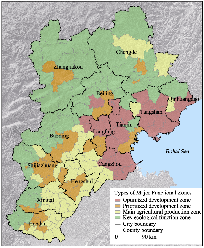
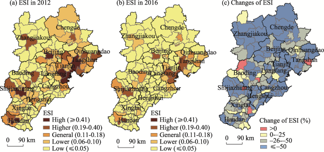
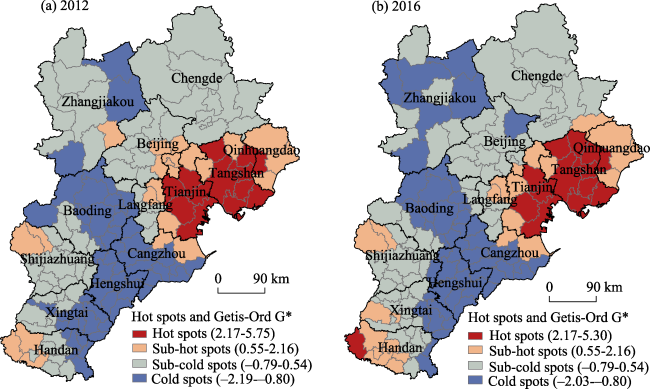
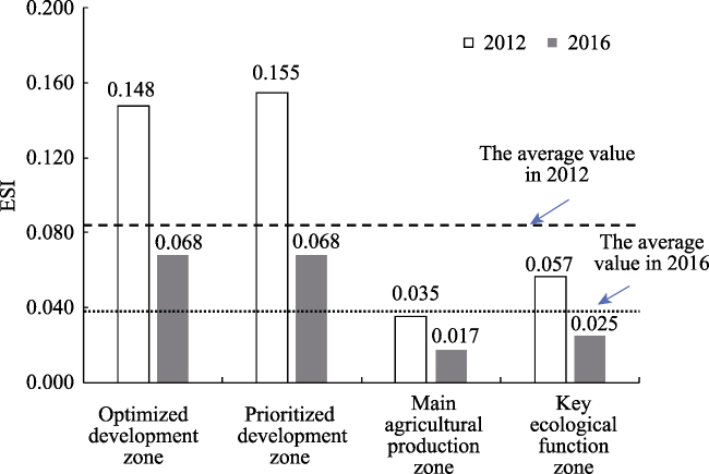
Environmental stress is used as an indicator of the overall pressure on regional environmental systems caused by the output of various pollutants as a result of human activities. Based on the pollutant emissions and socioeconomic databases of the counties in Beijing-Tianjin-Hebei region, this paper comprehensively calculates the environmental stress index (ESI) for the urban agglomeration using the entropy weight method (EWM) at the county scale and analyzes the spatiotemporal patterns and the differences among the four types of major functional zones (MFZ) for the period 2012-2016. In addition, the socioeconomic driving forces of environmental stress are quantitatively estimated using the geographically weighted regression (GWR) method based on the STIRPAT model framework. The results show that: (1) The level of environmental stress in the Beijing-Tianjin-Hebei region was significantly alleviated during that time period, with a decrease in ESI of 54.68% by 2016. This decrease was most significant in Beijing, Tangshan, Tianjin, Shijiazhuang, and other central urban areas, as well as the Binhai New Area. The level of environmental stress in counties decreased gradually from the central urban areas to the suburban areas, and the high-level stress counties were eliminated by 2016. (2) The spatial spillover effect of environmental stress increased further at the county scale from 2012 to 2016, and spatial locking and path dependence emerged in the cities of Tangshan and Tianjin. (3) Urbanized zones (development-optimized and development-prioritized zones) were the major areas bearing environmental pollution in the Beijing-Tianjin-Hebei region in that time period. The ESI accounted for 65.98% of the whole region, where there was a need to focus on the prevention and control of environmental pollution. (4) The driving factors of environmental stress at the county scale included population size and the level of economic development. In addition, the technical capacity of environmental waste disposal, the intensity of agricultural production input, the intensity of territorial development, and the level of urbanization also had a certain degree of influence. (5) There was spatial heterogeneity in the effects of the various driving factors on the level of environmental stress. Thus, it was necessary to adopt differentiated environmental governance and reduction countermeasures in respect of emission sources, according to the intensity and spatiotemporal differences in the driving forces in order to improve the accuracy and adaptability of environmental collaborative control in the Beijing-Tianjin-Hebei region.
ZHOU Kan , YIN Yue , LI Hui , SHEN Yuming . Driving factors and spatiotemporal effects of environmental stress in urban agglomeration: Evidence from the Beijing-Tianjin-Hebei region of China[J]. Journal of Geographical Sciences, 2021 , 31(1) : 91 -110 . DOI: 10.1007/s11442-021-1834-z
Figure 1 Distribution map showing the location of the Beijing-Tianjin-Hebei region the major functional zones (MFZ) |
Table 1 Emission intensity and ESI in the Beijing-Tianjin-Hebei region in 2012 and 2016 |
| Area | 2012 | 2016 | |||||||||
|---|---|---|---|---|---|---|---|---|---|---|---|
| COD (t) | NH3-N (t) | SO2 (t) | NOx (t) | ESI | COD (t) | NH3-N (t) | SO2 (t) | NOx (t) | ESI | ||
| Beijing | 16954.62 | 1862.13 | 8531.76 | 8876.63 | 0.10 | 7917.70 | 506.92 | 3019.09 | 3191.49 | 0.04 | |
| Tianjin | 32776.27 | 3630.82 | 32074.49 | 40024.72 | 0.28 | 14753.91 | 2235.31 | 10087.73 | 13820.09 | 0.12 | |
| Hebei | 9933.54 | 814.72 | 9871.90 | 8921.88 | 0.07 | 3023.46 | 451.93 | 5804.73 | 4786.54 | 0.03 | |
| Beijing- Tianjin- Hebei region | 11473.35 | 1017.54 | 10785.39 | 10332.41 | 0.08 | 3906.25 | 536.92 | 5800.44 | 5083.22 | 0.04 | |
Figure 2 ESI and its spatial changes in the Beijing-Tianjin-Hebei region in 2012 and 2016 |
Table 2 Moran’s I of ESI and major pollutants in the Beijing-Tianjin-Hebei region |
| Indicator | 2012 | 2016 | ||||
|---|---|---|---|---|---|---|
| Moran’s I | z-score | p-value | Moran’s I | z-score | p-value | |
| COD | 0.1666 | 3.6114 | 0.0003 | 0.1309 | 2.9777 | 0.0029 |
| NH3-N | 0.1592 | 3.6328 | 0.0003 | 0.1933 | 4.4142 | 0.0000 |
| SO2 | 0.2186 | 4.8671 | 0.0000 | 0.1865 | 4.1760 | 0.0000 |
| NOx | 0.1847 | 4.0896 | 0.0000 | 0.2720 | 5.9211 | 0.0000 |
| ESI | 0.2014 | 4.3945 | 0.0000 | 0.2325 | 5.0628 | 0.0000 |
Figure 3 Spatial changes in ESI in cold and hot spots in the Beijing-Tianjin-Hebei region in 2012 and 2016 |
Figure 4 The ESI of major functional zones in the Beijing-Tianjin-Hebei region in 2012 and 2016 |
Table 3 Estimated results of the OLS model in the Beijing-Tianjin-Hebei region |
| Variable | 2012 | 2016 | ||||||||
|---|---|---|---|---|---|---|---|---|---|---|
| Coefficient | Standard error | T statistic | P value | VIF | Coefficient | Standard error | T statistic | P value | VIF | |
| Intercept | -0.1521** | 0.0200 | -7.5971 | 0.0000 | — | -0.1939** | 0.0232 | -8.3752 | 0.0000 | — |
| TP | 0.8183** | 0.0691 | 11.8378 | 0.0000 | 1.9735 | 0.6341** | 0.0764 | 8.2948 | 0.0000 | 2.0188 |
| PGDP | 0.7390** | 0.0684 | 10.8029 | 0.0000 | 1.4166 | 0.6220** | 0.0764 | 8.1423 | 0.0000 | 1.3983 |
| IS | 0.0413 | 0.0277 | 1.4900 | 0.1062 | 1.1709 | 0.0763* | 0.0324 | 2.3520 | 0.0034 | 1.2015 |
| TDI | -0.1650** | 0.0498 | -3.3139 | 0.0044 | 2.4017 | -0.1347** | 0.0543 | -2.4799 | 0.0131 | 2.3414 |
| ETT | 0.3260** | 0.0351 | 9.2818 | 0.0000 | 1.0524 | 0.3028** | 0.0319 | 9.4878 | 0.0000 | 1.0906 |
| UR | 0.2135** | 0.0346 | 6.1780 | 0.0001 | 2.0578 | 0.2630** | 0.0378 | 6.9495 | 0.0001 | 2.0217 |
| IAP | 0.2802** | 0.0326 | 8.5851 | 0.0002 | 1.0872 | 0.2515** | 0.0349 | 7.1992 | 0.0007 | 1.1159 |
| Model diagnosis | Chi-square statistics | Correction R² | AIC | K(BP) test | Jarque- Bera test | Chi-square statistics | Correction R² | AIC | K(BP) test | Jarque- Bera test |
| 1277.1215 | 0.8469 | -411.5215 | 33.50139** | 3816.7202** | 996.9724 | 0.7847 | -376.3448 | 31.2104** | 3411.6170** | |
Note: ** is significant at the 0.01 level and * is significant at the 0.05 level. |
Table 4 Estimated results of the GWR model for the Beijing-Tianjin-Hebei region |
| Variable | 2012 | 2016 | |||||||||||
|---|---|---|---|---|---|---|---|---|---|---|---|---|---|
| Minimum value | Maximum value | Average value | Upper quartile | Median | Lower quartile | Minimum value | Maximum value | Average value | Upper quartile | Median | Lower quartile | ||
| Intercept | -0.407 | -0.035 | -0.137 | -0.170 | -0.094 | -0.073 | -0.399 | -0.084 | -0.169 | -0.197 | -0.146 | -0.122 | |
| TP | 0.658 | 2.896 | 1.307 | 0.798 | 1.083 | 1.655 | 0.420 | 2.985 | 1.055 | 0.571 | 0.867 | 1.306 | |
| PGDP | -1.277 | 2.071 | 0.973 | 0.704 | 0.749 | 1.540 | 0.020 | 3.405 | 0.868 | 0.554 | 0.607 | 0.936 | |
| IS | -0.052 | 0.244 | 0.032 | -0.020 | 0.007 | 0.060 | -0.040 | 0.345 | 0.071 | 0.026 | 0.047 | 0.094 | |
| TDI | -1.110 | 0.052 | -0.145 | -0.144 | -0.095 | -0.058 | -0.377 | 0.088 | -0.074 | -0.107 | -0.062 | -0.022 | |
| ETT | 0.150 | 0.621 | 0.327 | 0.210 | 0.293 | 0.429 | 0.171 | 0.486 | 0.275 | 0.227 | 0.252 | 0.302 | |
| UR | -0.004 | 0.459 | 0.136 | 0.076 | 0.097 | 0.165 | 0.004 | 0.352 | 0.157 | 0.110 | 0.144 | 0.197 | |
| IAP | -0.165 | 0.918 | 0.202 | 0.014 | 0.161 | 0.395 | -0.119 | 0.544 | 0.182 | 0.028 | 0.161 | 0.301 | |
| Model diagnosis | Bandwidth | Correction R² | AIC | Bandwidth | Correction R² | AIC | |||||||
| 99877.656 | 0.948 | -527.574 | 105540.116 | 0.900 | -454.605 | ||||||||
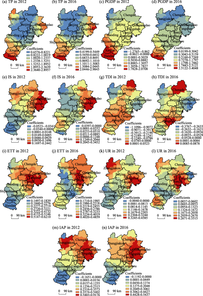
Figure 5 Spatial distribution of regression coefficients in the Beijing-Tianjin-Hebei region |
| [1] |
|
| [2] |
|
| [3] |
|
| [4] |
|
| [5] |
|
| [6] |
|
| [7] |
|
| [8] |
|
| [9] |
|
| [10] |
|
| [11] |
|
| [12] |
|
| [13] |
|
| [14] |
|
| [15] |
|
| [16] |
|
| [17] |
|
| [18] |
|
| [19] |
|
| [20] |
|
| [21] |
|
| [22] |
|
| [23] |
|
| [24] |
|
| [25] |
|
| [26] |
|
| [27] |
|
| [28] |
|
| [29] |
|
| [30] |
|
| [31] |
|
| [32] |
|
| [33] |
|
| [34] |
|
| [35] |
|
| [36] |
|
| [37] |
|
| [38] |
|
| [39] |
|
| [40] |
|
| [41] |
|
/
| 〈 |
|
〉 |