Regular Research Articles

Vertical differentiation of land cover in the central Himalayas

  • ZHANG Yili 1, 2, 3 ,
  • WU Xue 1, 3 ,
  • ZHENG Du 1
Expand
  • 1. Key Laboratory of Environment Change and Resources Use in Beibu Gulf, the Ministry of Education, Nanning Normal University, Nanning 530001, Guangxi, China
  • 2. CAS Center for Excellence in Tibetan Plateau Earth Sciences, Beijing 100101, China
  • 3. University of Chinese Academy of Sciences, Beijing 100049, China

Zhang Yili and Wu Xue are co-first authors. E-mail: wuxuexxl@163.com; zhangyl@igsnrr.ac.cn

Received date: 2020-02-22

  Accepted date: 2020-04-06

  Online published: 2020-08-25

Supported by

National Natural Science Foundation of China(No.41761144081)

The Priority Research Program of Chinese Academy of Sciences(No.XDA20040201)

The Second Tibetan Plateau Scientific Expedition and Research(No.2019QZKK0603)

Copyright

Copyright reserved © 2020.

Abstract

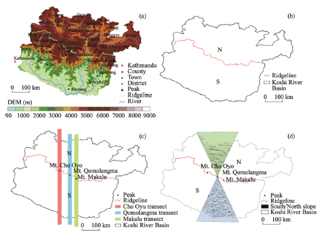
Characterized by obvious altitudinal variation, habitat complexity, and diversity in land cover, the Mt. Qomolangma region within the central Himalayas is one of the most sensitive areas to climate change in the world. At the same time, because the Mt. Qomolangma region possesses the most complete natural vertical spectrum in the world, it is also an ideal place to study the vertical structure of alpine land cover. In this study, land cover data for 2010 along with digital elevation model data were used to define three methods for dividing the northern and southern slopes in the Mt. Qomolangma region, i.e., the ridgeline method, the sample transect method, and the sector method. The altitudinal distributions of different land cover types were then investigated for both the northern and southern slopes of the Mt. Qomolangma region by using the above three division methods along with ArcGIS and MATLAB tools. The results indicate that the land cover in the study region was characterized by obviously vertical zonation with the south-six and north-four pattern of vertical spectrum that reflected both the natural vertical structure of vegetation and the effects of human activities. From low to high elevation, the main land cover types were forests, grasslands, sparse vegetation, bare land, and glacier/snow cover. The compositions and distributions of land cover types differed significantly between the northern and southern slopes; the southern slope exhibited more complex land cover distributions with wider elevation ranges than the northern slope. The area proportion of each land cover type also varied with elevation. Accordingly, the vertical distribution patterns of different land cover types on the southern and northern slopes could be divided into four categories, with glaciers/snow cover, sparse vegetation, and grasslands conforming to unimodal distributions. The distribution of bare land followed a unimodal pattern on the southern slope but a bimodal pattern on the northern slope. Finally, the use of different slope division methods produced similar vertical belt structures on the southern slope but different ones on the northern slope. Among the three division methods, the sector method was better to reflect the natural distribution pattern of land cover.

Cite this article

ZHANG Yili , WU Xue , ZHENG Du . Vertical differentiation of land cover in the central Himalayas[J]. Journal of Geographical Sciences, 2020 , 30(6) : 969 -987 . DOI: 10.1007/s11442-020-1765-0

1 Introduction

Human beings affect the land surface by changing the land cover (Haberlet al., 2007). Changes in land cover and the ecological environment are considered to be a key issue by numerous international organizations and scientific research programs (Pitman et al., 2011; He et al., 2014), and are thus a key area of study in global change research (Mooney et al., 2013). Under certain conditions, the gradient of natural zones in the vertical direction is 1000 times that in the horizontal direction (Walter, 1973). The study of natural mountain belts is an effective way to reveal the complexity and heterogeneity of mountain environments. The changes in vertical zonation are an important indicator of climate change (Dullinger, 2004). Accordingly, numerous comparative studies have been carried out on the vertical spatial patterns in mountainous regions worldwide, including comparative analyses of snow lines and the upper/lower limits of forests (Walter, 1973; Allan, 1986; Callaway, 1997). In alpine environments, climate change has been shown to affect plant physiological processes, species composition, and the diversity of plant communities, which may change the structures and functional characteristics of these communities. The transitional zone or ecotone between different vegetation types is particularly sensitive to the effects of climate change. For example, in the Alps, the mountains of North America (Grabherr et al., 1994), and Wutai Mountain (Mu, 2003), observed changes include the vertical movement of the boundary line of vegetation, the increase in the altitude of the alpine forest line (Beniston, 2003), and the change in plant growth at the polar forest line (Gian-Reto et al., 2002; Liang et al., 2016). Some studies have explored the spatial relationship between climate change and vertical belts through statistical analysis, simulation, and field studies. For example, Xu et al. (2009) investigated the spatial relationship between mountain vertical belts and climate factors, Yao et al. (2015) studied the effect of warming on vertical zonation, and Liang et al. (2016) and Li et al. (2016) reported the mechanisms of the responses of the forest line and tree line to climate change.
Mt. Qomolangma (MQ), located in the middle of the Himalayas, has a large elevation range, complex habitat, and unique ecosystem types (Cidanlunzhu, 1997). MQ also possesses the world’s most complete natural vertical zonation, making it an ideal place to study the vertical changes in high-altitude vegetation. In the 1970s, Zhang and Jiang (1973) systematically analyzed the relationship between vertical zonal vegetation and horizontal zonal vegetation in the MQ area based on data collected by the scientific expedition team of the Chinese Qomolangma Mountaineering Team (1959-1960), the Tibetan Comprehensive Expedition Team of the Chinese Academy of Sciences (1960-1961), and the Tibet Scientific Expedition of the Chinese Academy of Sciences (1966-1968). In the 1980s, Zheng (1981) further clarified the vertical characteristics of vegetation in the eastern Himalayas. These studies have had a profound influence on our understanding of the vertical zonation and three-dimensional zonal characteristics of vegetation in the MQ region along with the patterns of vertical differentiation in the natural environment.
Due to the limitation of research conditions, most previous studies on mountain vertical belts were only based on limited field survey data or other data with low temporal and spatial continuity. In addition, these studies mainly focused on a single or few types of vertical belt boundaries (e.g., forest line and snow line). Few studies have analyzed the vertical zonation of entire mountains. A single point or a single line (spatial location) was often used to represent the boundary in the vertical zone, weakening the transition characteristics of the vertical zone boundary. While such a simple linear band structure can describe the vertical characteristics of vegetation, it cannot provide information about the formation process of mountain vertical belts, resulting in uncertainty regarding the evolution of vertical zones. This study explores the vertical structure and distribution of land cover on the southern and northern slopes of the central Himalayas using high-resolution land cover data and geographic information system (GIS) spatial analysis. Revealing the spatial differentiation of land cover on the southern and northern slopes of the central Himalayas, this study also provides a new method for studying vertical zonation in mountain regions.

2 Methodology

The study area was located in the upper and middle reaches of the Koshi River Basin (KRB) in the middle of the Himalayas in China and Nepal, with a geographical position of 85°22'-88°21'E, 26°47'-29°12'N. The KRB extends to the south of the Yarlung Zangbo River in the north, borders between Nepal and India on the south, the vicinity of Kathmandu in the west, and the borders between China, Nepal and India to the east (Figure 1a), covering a total area of 53,988.4 km2 (Zhang et al., 2013). The average elevation of the KRB is 3783 m, and more than 49% of the area of the KRB lies above 4500 m. The KRB includes six major peaks, i.e., MQ (8844 m), Mt. Makalu (MM, 8463 m), Mt. Cho Oyu (MC, 8201 m), Mt. Kanchenjunga (MK, 8586 m), Mt. Lhotse (8516 m), and Mt. Xixiabangma (8012 m) (Zhang et al., 2013; Wu et al., 2017). Valleys are distributed among the mountains in the KRB, and include the Boqu valley, Rongxia valley and Pengqu valley in China from west to east.
Figure 1 Maps of the study area showing the terrain (a), and the southern and northern slopes of Mt. Qomolangma determined by using three division methods: (b) ridgeline method, (c) sample transect method and (d) sector methodZ

2.1 Data

The data used in this study were land cover data and topographic data for 2010. The land cover data were provided by the Land Change and Regional Adaptation Research Group of the Tibetan Plateau, Institute of Geographic Sciences and Natural Resources Research, CAS (Wu et al., 2017). The spatial resolution of the data was 30 m. The Class-I land cover type interpretation accuracy was between 71% and 100% with an average of 83.36%. Digital elevation model (DEM) data (ASTER GDEM) were obtained from the Unites States Geological Survey network at a resolution of 30 m (https://earthexplorer.usgs.gov). Other topographic data were derived from the DEM data.

2.2 Methods

2.2.1 Division of the southern and northern slopes
To analyze the vertical distribution characteristics of land cover, the formation process of vertical belts, and the similarities and differences in vertical zonation on the southern and northern slopes in the study area, it is necessary to accurately depict the distributions and structural characteristics of land cover types on two slopes. Accordingly, the following three division methods were used to divide the southern and northern slopes, allowing the analysis of the vertical distribution of land cover on each slope:
(1) Ridgeline method. In this conventional method, the southern and northern slopes were divided by using the ridgeline of the Himalayas as a boundary. The ridgeline was expressed as a single line from the bottom of the mountain to the top on the southern or northern slope. Based on this division method, the southern slope included all the mountains and their slopes, which are lower than the Himalayan ridge, and so is the northern slope. The areas of the southern and northern slopes in the study area were shown in Figure 1b.
(2) Sample transect method. In this method, the peak of each mountain was taken as an apex, with 0° direction as the northern slope and 180° direction as the southern slope. The slope direction was divided according to the degree of sunlight received. The southern slope included all the mountains and their land cover types of each slope direction in sample transect, as well as the northern slope. To study the vertical distribution of land cover in high-altitude mountains, three rectangular transects (bandwidth = 10 km) of the southern and northern slopes spanning MQ, MC, and MM were created in this study (Figure 1c). These transects were referred to as the MQ transect, MC transect, and MM transect, respectively.
(3) Sector method. In this method, the peak of the mountain was taken as the apex, and the area within 157.5° southeast-180° south-202.5° southwest was taken as the southern slope, while the area within 337.5° northwest-0° north-22.5° northeast was taken as the northern slope. The southern (northern) slope included the southern (northern) slopes of all mountains. The southern slope of the mountain was the southern slope of the sector, while the northern slope of the mountain was the northern slope of the sector. The MQ region was selected as the research sample area (Figure 1d).
2.2.2 Extraction of land cover data using ArcGIS and MATLAB
The land cover data for the study area were extracted as follows. For the ridgeline method, the ridge of the main Himalayan Mountains was taken as the boundary to divide the northern and southern slopes. The aspect tool in ArcGIS was then used to extract the data for the southern and northern slope areas. The divided southern and northern slope areas were then used as masks to extract the land cover type data for each slope.
2.2.3 Statistical analysis of the vertical distribution of land cover
MATLAB was used to obtain the vertical land cover data. The extracted land cover and elevation data for the northern and southern slopes were converted into ASCII format. MATLAB was then used to overlay the land cover and elevation data to calculate the proportions of different land cover types using a 100-m gradient range.
2.2.4 Definition of relevant terms
To get a better understanding of the spatial structure and characteristics of the vertical zones of land cover, the following terms were defined.
Distribution of upper limit/lower limit referred to the elevation zone of the uppermost/lowermost edge of the continuous distribution of a land cover type (Figure 2). In the actual operation, if the complete pixel information of the land cover type appeared in a 100-meter vertical distribution band, this land cover type was considered to be present. If the 100-meter zone was the highest altitude of the distribution of the land cover type, the elevation zone was regarded as the upper limit of that type; while if the 100-meter zone was the lowest altitude of the distribution of the land cover type, the elevation zone was regarded as the lower limit of that type.
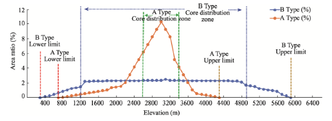
Figure 2 Schematic showing the terminology used to describe the altitudinal distributions of land cover types
Core distribution zone (core distribution range) was related to the elevation range of a land cover type in its vertical distribution, with the number of elevation zones accounting for less than one-third of the total elevation zones within the distribution range of this land cover type, and the distribution area accounting for more than two-thirds of the total distribution area (Figure 2). The entire vertical distribution range of this land cover type that accounted for less than one-third of its total distribution zone was defined as the core distribution range of this land cover type. The interval of its elevation distribution zone was called the core distribution zone. The core distribution zone and core distribution range were determined as follows. The elevation zone with the largest area proportion of this land cover type was taken as the center, and the area was extended from the center to both sides (up and down) with equal area ratio. When the area proportion of this land cover type was more than two-thirds of the total area of the land cover type, its vertical distribution range was considered to be the core distribution range of this land cover type, and its elevation distribution interval was considered as the core distribution zone. The core distribution zone referred to as the distribution range and proportion of the land cover type with an area proportion of 100%.
Main distribution zone. If land cover type had no obvious core distribution zone in its vertical distribution range, the vertical distribution area accounted for over two-thirds of the area of that land cover type (Figure 2). In application, if the area was increased from the zone with the largest area ratio of vertical distribution zone to both sides (up and down) with equal area ratio, and the distribution area ratio accounted for more than two-thirds of the total distribution area of this type, the vertical distribution range of this type was defined as the main distribution zone of this land cover type, and the elevation zone interval was called the main distribution zone of this type. This referred to the distribution range and proportion of the land cover type with an area proportion of 100%.
Dominant belt referred to the elevation interval in which the proportion of the distribution area of one land cover type was absolutely dominant over other land cover types (over two-thirds of the area of the elevation belt). Generally, dominant belt also referred to the distribution interval with the highest area proportion of a land cover type in each elevation zone. In the vertical distribution, the dominant zones of each type were distributed alternately and did not overlap.
Compound dominant zone referred to the case where there was no absolute predominance of a certain land cover type within a certain elevation range; instead, two or three land cover types had similar area proportions and distributions within an elevation interval. In this case, compound dominant zone referred to the combination of these two or three land cover types (Figure 3), and the naming convention was based on the area proportions in the zone. For example, considering a certain elevation range in which the area proportions of shrubland and grassland are 52% and 42%, respectively, the compound dominant zone was called the shrubland-grassland dominant zone. Alternatively, for an elevation zone consisting of 30% shrubland area, 31% forest area, 29% farmland area, and 10% construction area, respectively, the compound dominant zone was called the forest-shrubland-farmland dominant zone.
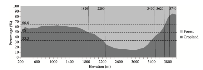
Figure 3 Schematic showing the vertical distributions of compound dominant land cover types (from left to right: cropland-forest dominant belt, forest-cropland dominant belt, forest dominant belt, forest-cropland dominant belt, cropland-forest dominant belt, and cropland dominant belt)
According to the changes in the area proportion of each land cover type with elevation, along with the shape, number, and location of the peak area of the area ratio distribution between the northern and southern slopes for each land cover type, the distribution of each land cover type on each slope was classified as one of the following four types:
1) Uni-no: one peak was observed in the area proportion curve of one land cover type on the southern or northern slope. Meanwhile, no obvious peak was observed on the other slope (e.g., a unimodal peak on the southern slope and no peak on the northern slope).
2) Unimodal: one peak was observed in the area proportion curve for one land cover type on both the southern and northern slopes. Based on the peak elevations, this category could be divided into “unimodal south-low and north-high” and “unimodal south-north uniform” patterns.
3) Unimodal-bimodal: one peak in the area proportion curve of one land cover type was observed on the southern or northern slope while two peaks are observed on the other slope. This type could be further divided into “south-unimodal and north-bimodal” and “south- bimodal and north unimodal” patterns.
4) Bimodal: one peak in the area proportion curve of one land cover type was observed on each slope (i.e., “north-south bimodal” pattern).

3 Results and analysis

3.1 Land cover types and characteristics

The land cover types in the KRB included 10 Class I types and 21 Class II types (Zhang et al., 1973). Ten Class I types were construction land, cropland, wetland, waterbody, forest, shrubland, grassland, sparse vegetation, bare land, and glacier and permanent snow cover, which was called glacier/snow cover for short. With an elevation ranging from 96 to 8844 m, there are 10 Class I types and 21 Class II types. The main land cover types were forest, shrubland, waterbody, cropland, and construction land. With an elevation ranging from 2100 to 8844 m, there are 7 to 10 Class I types and 10 to 20 Class II types on the northern slope. The land cover types on the northern slope were mainly grassland, sparse vegetation, wetland, and bare land. In the three methods used to divide the southern and northern slopes, the Class I land cover types on the southern slope were basically the same. In contrast, on the northern slope, 2 to 3 main land cover types were not found at low elevation if the sample transect or sector method was used to divide the slopes compared to that if the ridgeline method was used. Meanwhile, if the ridgeline method was used, the northern slope was missing one Class II land cover type compared with the southern slope. Based on the sample transect and sector methods, the northern slope contained only 10 (or 11) Class II land cover types, 9 (or 10) less than that obtained using the ridgeline method. These results reflected the distribution characteristics of land cover in the high-altitude area of the northern slope.
The southern slope in the KRB had a slightly larger area than the northern slope (Table 1). The land cover types on the southern slope were mainly forest and cropland, which accounted for 60%-86% of the area of the southern slope. The northern slope was dominated by grassland and bare land, which accounted for 74%-80% of the northern slope’s area. The results obtained using the sector method are as follows. The southern slope was dominated by forests and cropland, these two types had similar area proportions and accounted for approximately 86% of the total area of the southern slope (Table 1). The northern slope was dominated by grassland, with an area proportion of 63% of the northern slope’s area, followed by bare land and sparse vegetation with area proportions of 16.33% and 12.89%, respectively. The area proportion of glacier/snow cover on the northern slope was higher than that on the southern slope. The results of the sample transect method are as follows. The southern slope was dominated by cropland and forest accounting for 60%-75% of the southern slope’s area; while the northern slope was dominated by grassland and bare land (73%). The area of glacier/snow cover was larger on the northern slope than on the southern slope. The results of the ridgeline method are as follows. The southern slope was dominated by forest, cropland, and glacier/snow cover; while the northern slope was mainly covered with grassland, bare land, and glacier/snow cover. The area of grassland was much higher (6.7 times higher) on the northern slope than on the southern slope; while forest was mainly distributed on the southern slope (Table 1).
Table 1 Areas and proportions of different land cover types on the northern and southern slopes
Land cover type Division method Southern slope Northern slope Area ratio
Area (km2) Percentage Area (km2) Percentage Southern slope: northern slope
Cropland Sector method 374.20 44.94 5.66 1.05 66.11︰1
MM transect 304.75 27.24 23.35 2.08 13.05︰1
MQ transect 240.29 19.52 8.21 0.87 29.27︰1
MC transect 406.96 31.88 9.04 1.02 45.02︰1
Ridgeline method* 7917.95 26.91 243.64 0.99 32.50︰1
Forest Sector method 342.38 41.12 - - -
MM transect 516.34 46.16 - - -
MQ transect 559.99 45.50 - - -
MC transect 406.80 31.87 - - -
Ridgeline method 11177 37.99 262.54 1.08 42.60︰1
Shrubland Sector method 13.62 1.64 - - -
MM transect 38.65 3.45 10.41 0.93 3.71︰1
MQ transect 34.85 2.83 - - -
MC transect 36.13 2.83 - - -
Ridgeline method 1433.42 4.87 660.56 2.69 2.17︰1
Grassland Sector method 22.17 2.66 340.08 62.99 0.07︰1
MM transect 41.97 3.75 553.23 49.38 0.08︰1
MQ transect 43.26 3.51 522.06 55.10 0.08︰1
MC transect 106.15 8.31 450.42 50.94 0.24︰1
Ridgeline method 2041.39 6.94 11886.72 48.40 0.17︰1
Sparse vegetation Sector method 10.16 1.22 69.57 12.89 0.15︰1
MM transect 28.04 2.51 96.74 8.63 0.29︰1
MQ transect 28.56 2.32 72.77 7.68 0.39︰1
MC transect 66.06 5.17 35.49 4.01 1.86︰1
Land cover type Division method Southern slope Northern slope Area ratio
Area (km2) Percentage Area (km2) Percentage Southern slope: northern slope
Ridgeline method 1016.77 3.46 1073.82 4.37 0.95︰1
Waterbody Sector method 9.50 1.14 0.01 0.00 950︰1
MM transect 9.67 0.86 6.90 0.62 1.40︰1
MQ transect 7.90 0.64 1.43 0.15 5.52︰1
MC transect 13.69 1.07 2.40 0.27 5.70︰1
Ridgeline method 182.87 0.62 152.43 0.62 1.20︰1
Construction land Sector method 0.32 0.04 1.17 0.22 0.27︰1
MM transect 0.19 0.02 0.48 0.04 0.40︰1
MQ transect - - - - -
MC transect - - - - -
Ridgeline method 13.68 0.05 0.79 0.00 17.30︰1
Bare land Sector method 34.37 4.13 88.18 16.33 0.39︰1
MM transect 87.34 7.81 277.88 24.80 0.31︰1
MQ transect 176.45 14.34 192.32 20.30 0.92︰1
MC transect 145.79 11.42 203.95 23.06 0.71︰1
Ridgeline method 4010.33 13.63 7750.94 31.56 0.52︰1
Wetland Sector method 3.18 0.38 14.93 2.77 0.21︰1
MM transect 8.35 0.75 12.86 1.15 0.65︰1
MQ transect 9.07 0.74 22.95 2.42 0.40︰1
MC transect 11.91 0.93 81.77 9.25 0.15︰1
Ridgeline method 279.49 0.95 787.95 3.21 0.36︰1
Glacier/snow cover** Sector method 22.83 2.74 20.26 3.75 1.13︰1
MM transect 83.27 7.44 138.51 12.36 0.60︰1
MQ transect 130.48 10.60 127.74 13.48 1.02︰1
MC transect 83.11 6.51 101.19 11.44 0.82︰1
Ridgeline method 1355.58 4.61 1740.59 7.09 0.78︰1
Total Sector method 832.73 100.00 539.87 100.00 1.54︰1
MM transect 1118.57 100.00 1120.36 100.00 1.00︰1
MQ transect 1230.85 100.00 947.48 100.00 1.30︰1
MC transect 1276.59 100.00 884.27 100.00 1.44︰1
Ridgeline method 29428.43 100.00 24559.97 100.00 1.20︰1

* Data for the ridgeline method were updated on the basic data of Wu et al. (2017). ** Glaciers and permanent snow cover.

3.2 Vertical distributions of different land cover types on the northern and southern slopes

The distributions of the various land cover types changed with the environmental gradient. Figure 4 shows the vertical distributions of different land cover types and their area proportions based on the three slope division methods. The vertical distribution patterns of land cover types on the northern and southern slopes were divided into four major categories and five minor categories as follows.
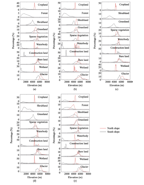
Figure 4 Altitudinal distributions of different land cover types on the southern and northern slopes based on the three slope division methods: (a) sector method; (b) MM sample transect method; (c) MQ sample transect method; (d) MC sample transect method; and (e) ridgeline method
1) South unimodal and north no peak pattern (MQ and MC sample transect methods and sector method). The elevation ranges obtained for forest (100-4000 m) and shrubland (1700-5100 m) on the southern slope were larger for the sector method than for the sample transect method, and peak values differed slightly. The forest distribution obtained using the sample transect method of MM belonged to this type. In the unimodal pattern, the peaks in the altitudinal distributions of some land cover types were significantly lower on the southern slope than on the northern slope. For example, the elevation distributions of glacier/snow cover on the southern slope of MQ obtained by the sector method and the sample transect method were 700 and 800 m lower than those of the northern slope, respectively. The distribution patterns of some land cover types, including grassland for the MQ sample transect method, cropland and sparse vegetation for the sector method, and forest, shrubland, cropland, and marsh wetland for the ridgeline method, could be described by “wide south and narrow north.” Due to the inclusion of multiple independent slope components in the ridgeline method, the distributions of grassland, sparse vegetation, and glacier/snow cover at high elevation nearly offset the difference in distribution between the northern and southern slopes. Therefore, the differences in distribution between the two slopes were not obvious in this case.
2) South-unimodal and north-bimodal pattern (a compound distribution of single and double peaks). For the three slope division methods, the peak value of bare land appeared in different positions on the northern and southern slopes. Sparse vegetation, marsh wetland, and cropland exhibited this pattern when the MQ sample transect method was used.
3) South-bimodal and north-unimodal pattern (a compound distribution of single and double peaks). The distributions of construction land based on the sector and ridgeline division methods and the distribution of waterbodies (rivers and lakes) based on the MQ sample transect method exhibited this pattern.
4) North-south bimodal pattern. The distribution of waterbodies (rivers and lakes) based on the sector division method belonged to this pattern. The two peaks in the distribution of water on the southern slope appeared in the elevation ranges of 200-300 m (accounting for 31% of the total area of waterbodies) and 4900-5000 m (4.9%). On the northern slope, the two peaks appeared in the elevation ranges of 4300-4400 m (38.2%) and 5200-5300 m (10.6%). The waterbodies in the high-elevation zone were mainly glacial lakes.
Regarding the distribution characteristics of single land cover types (Class I), with the exception of forest, which was mainly distributed on the southern slope, the vertical distribution ranges of all land cover types on the southern slope were wider than those on the northern slope, while the elevations of the distributions and the core distribution zones were lower on the southern slope than on the northern slope (Figure 4 and Table 2). The elevation ranges and core distribution zones also differ significantly among land cover types. The elevation ranges and core distribution zones on the southern slope are as follows (from low to high elevation): cropland (elevation range: 100-4000 m, core distribution zone: 500-2200 m); forest (100-4000 m, 500-3100 m); shrubland (300-5100 m, 3300-4600 m); grassland (1400-5900 m, 4100-5100 m); sparse vegetation (300-5300 m, 4100-5300 m), bare land (over 3000 m, 4300-5900 m), and glacier snow cover (over 4100 m, 4700-6000 m). In addition, waterbodies (100-5400 m, 100-5400 m), marsh wetlands (100-5200 m, 100-1400 m), and construction land (400-2400 m, 1000-1600 m) are distributed along the valleys (Table 2). On the northern slope, the elevation ranges and core distribution zones of each land cover type were as follows (from low to high elevation): cropland (4000-4600 m, 4000-4500 m); shrubland (4300-5300 m, 4500-5000 m); grassland (3900-5100 m, 4200-5000 m); sparse vegetation (4600-5400 m, 5000-5400 m); bare land (over 4200 m, 5000-5900 m); and glacier/snow cover (over 4300 m, 5200-6700 m). Waterbodies (4200-6100 m, 4200-5000 m), wetlands (3900-5500 m, 4000-4500 m), and construction land (4200-4400 m, 4300-4400 m) were distributed along the valleys.
Table 2 Altitudinal distributions of different land cover types on the northern and southern slopes based on different slope division methods
Land cover type Division method Southern slope Northern slope
Class I - Elevation range (m) Core distribution zone (m) Advantage
zone (m)
Elevation range (m) Core distribution zone (m) Advantage
zone (m)
Cropland Sector method 100-4000 600-1700 100-1800 4000-4500 4100-4500 -
MM transect 100-4000 1100-2200 1000-1700 4200-4600 4200-4500 -
MQ transect 100-4000 700-1500 - 3900-4500 4300-4500 -
MC transect 200-4000 500-1400 200-1400 4200-4500 4400-4500 -
Ridgeline
method
96-4300 700-1700 100-1500 2300-4500 4100-4500 -
Forest Sector method 100-4000 500-2000 1800-3600 - - -
MM transect 100-4000 1700-3100 100-1000
1700-3900
- - -
MQ transect 100-4000 600-1900 100-3700 - - -
MC transect 200-4000 700-2200 1400-3800 - - -
Ridgeline
method
100-4000 1100-2600 1500-3800 2100-4000 3200-4000 2300-3900
Shrubland Sector method 1700-5100 3300-4200 3600-4000 - - -
MM transect 1700-5000 3200-4200 3900-4100 - - -
MQ transect 1600-5000 3700-4200 3700-4200 4300-5300 4500-5000 -
MC transect 1600-5100 3500-4300 3800-4000 - - -
Ridgeline
method
300-4800 3400-4600 3800-4200 2400-4800 4200-4800 3900-4100
Grassland Sector method 1600-5900 4100-5100 4000-5000 4000-5100 4500-5000 4000-5100
MM transect 3000-5100 4600-5100 4200-5100 4400-4900 4200-5100
MQ transect 1500-5100 4100-5000 3900-5100 4400-5000 4000-5100
MC transect 2500-5100 4300-5000 4000-5000 4200-5100 4300-4700 4400-5000
Ridgeline
method
1400-5100 4400-5000 4400-5000 2500-5100 4400-5000 4100-5100
Sparse
vegetation
Sector method 3000-5300 4400-5300 - 4600-5400 5000-5400 5100-5400
MM transect 3000-5300 4500-5300 - 4700-5300 5000-5300 5100-5300
MQ transect 3300-5300 4100-4800 - 4700-5300 5200-5300 5100-5300
MC transect 3100-5300 4500-5200 - 4700-5300 5200-5300 5200-5300
Ridgeline
method
2100-5300 4600-5300 - 4000-5400 5000-5400 5100-5400
Waterbody Sector method 100-2500
4200-5300
100-500 - 4200-4500
5000-5800
4200-4400 -
MM transect 100-800
1400-2200
4600-5400
4900-5400 - 4200-4400
5700-6100
4200-4300 -
MQ transect 100-900
3700-5300
100-500 - 4200-5300 4200-4300
4800-5000
-
MC transect 200-1800
4200-5300
200-700 - 4200-4400
5500-5800
4300-4400 -
Ridgeline
method
96-2900
3700-5300
200-700
4900-5300
- 2200-5300 4100-4600 -
Construction land Sector method 1000-1700 1100-1300
1500-1600
- 4200-4400 4300-4400 -
MM transect - - - - - -
MQ transect 1500-1700 1500-1600 - 4200-4400 4300-4400 -
Land cover type Division method Southern slope Northern slope
Class I Elevation range (m) Core distribution zone (m) Advantage
zone (m)
Elevation range (m) Core distribution zone (m) Advantage
Zone (m)
MC transect - - - - - -
Ridgeline
method
400-2400 1000-1600 - 4200-4400 4200-4400 -
Bare land Sector method >3000 4800-5900 5000-5700 > 4200 5100-5600 5400-6000
MM transect >3000 5000-5900 4100-5500 > 4200 5000-5900 5300-6100
MQ transect >3400 4300-5200 4200-5100 > 4300 5100-5700 5300-5900
MC transect >3100 5000-5500 5000-5900 > 4300 5000-5800 5000-5200
5300-6100
Ridgeline
method
>1100 4700-5700 4200-4400
5000-5700
>3000 5000-5700 5400-6000
Wetland Sector method < 2800 100-500 - 4000-5000 4200-4500 -
MM transect < 4900 100-1000 - 4200-5200 4200-4500 -
MQ transect 100-4500 400-1100 - 3900-5300 4000-4400 3900-4000
MC transect < 5200 200-1400 - < 5500 4300-4400 -
Ridgeline
method
< 5100 200-1400 - 3500-5300 4100-4400 -
Glacier/snow cover Sector method > 4400 5200-5900 > 5700 > 5100 6000-6600 >6000
MM transect > 4800 5100-5800 > 5500 > 5400 6000-6700 >6100
MQ transect > 4100 5000-6000 > 5100 > 4300 5200-6300 > 5900
MC transect > 4600 4700-5700 > 5900 > 5400 6000-6600 >6100
Ridgeline
method
> 4000 5100-5900 > 5700 >3800 5400-6300 >6000

3.3 Vertical distribution characteristics of land cover types in the central Himalayas

The vertical distributions of land cover types on the southern slope were wider and the vertical zone spectrum was more complete; while the northern slope was dominated by high-elevation land cover types with narrower distributions (Figure 5). The vertical distributions of land cover differed between the southern and northern slopes. Construction land and cropland, which were related to human activities, were mostly distributed along mountains and valleys (rivers) in a wide range of elevations. At low and middle elevations, construction land and cropland were often crisscrossed by forests and shrubland; thus, the vertical distribution of land cover in the KRB had characteristics affected by human activities. The distributions and compositions of different land cover types on the southern and northern slopes were graphically depicted in Figure 5. On the southern slope, forest, shrubland, grassland, sparse vegetation, bare land, and glacier/snow cover exhibited zonal distributions; while cropland, construction land, wetland, and waterbodies were distributed in a wide range of elevation (Figure 5). The result of using three methods for dividing the northern and southern slopes showed the characteristics of this land cover type’s composition to some extent; only the elevation and area of its distribution were different. On the northern slope, cropland, grassland, sparse vegetation, bare land, and glacier/snow cover showed zonal distributions; while cropland and construction land were distributed in the valleys below 4400 m. Wetland was distributed together with waterbodies or distributed along the edges of glacier/snow cover.
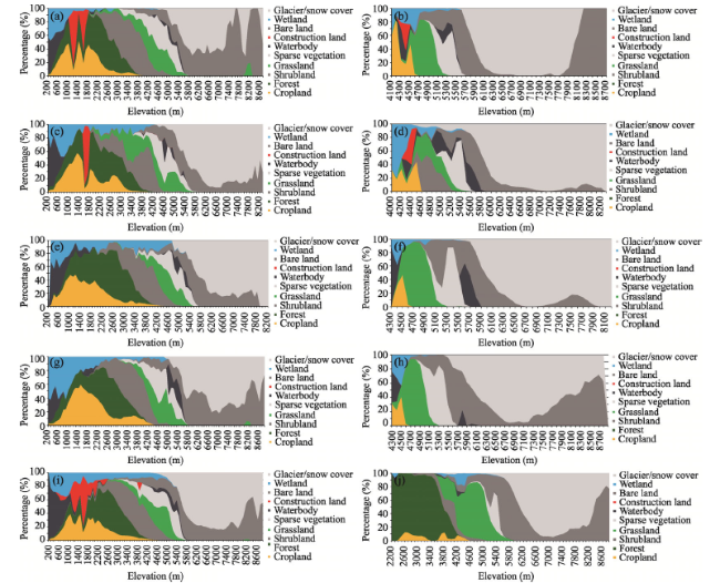
Figure 5 Distributions and compositions of different land cover types in different vertical zones on the northern and southern slopes based on different slope division methods: (a) southern slope, sector method; (b) northern slope, sector method; (c) southern slope, MM sample transect method; (d) northern slope, MM sample transect method; (e) southern slope, MC sample transect method; (f) northern slope, MC sample transect method; (g) southern slope, MQ sample transect method; (h) northern slope, MQ sample transect method; (i) southern slope, ridgeline method; and (j) northern slope, ridgeline method
From low to high elevation, the land cover type composition changed from complex to simple (i.e., from three or four land cover types to one type on the southern slope and from two or three land cover types to one type on the northern slope; Figure 5). The land cover type composition changed with elevation, reflecting comprehensive results of ecosystem adaptation and human influence.
To clearly explain the vertical distribution characteristics of land cover types in the study region, Figure 6 graphically shows the vertical belts of land cover types (Class I) for both the southern and northern slopes (Table 2). Figure 6 indicates a “south six, north four (five)” vertical belt pattern in the middle Himalayas (Figures 6a and 6b). In this pattern, “south six” referred to cropland, forest, shrubland, grassland, bare land, and glacier/snow cover; while “north four (five)” referred to (wetland), grassland, sparse vegetation, bare land, and glacier/snow cover. This structure reflected the internal relationship between land cover and the vertical natural zones on MQ. The distribution of cropland or cropland-forest composite belt on the southern slope (Figure 6b) also reflected the effects of human activities.
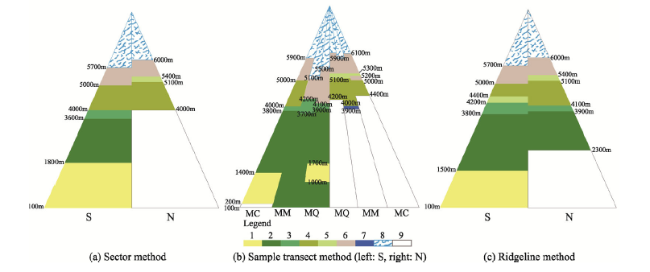
Figure 6 Dominant altitudinal band structures of land cover types on the southern and northern slopes of the KRB based on different slope division methods: (a) sector method; (b) sample transect method with MQ, MC, and MM transects; and (c) ridgeline method. For the ridgeline method, both the southern and northern slopes contain unique distribution types in the two directions, which increase the uncertainty in the results. Therefore, the vertical zonation of land cover based on the ridgeline method is not discussed in this paper.

Note: code representation in legend: 1-cropland, 2-forest, 3-shrubland, 4-grassland, 5-sparse vegetation, 6-bare land, 7-waterbody, 8-glacier/snow cover, 9-none

4 Discussion

4.1 Relationships between the vertical distribution of land cover and the distributions of climatic and soil zones

Due to the huge differences in topography in the MQ region, the hydrothermal conditions changed with elevation, and obvious vertical changes in climate, soil, and ecosystems were observed. The climate and soil types on MQ differed significantly between the northern and southern slopes (Table 3) (Tibet Scientific Expedition Team of the Chinese Academy of Sciences, 1975). Comparison of the vertical distributions of land cover types with the vertical distributions of climate and soil types showed that the northern and southern slopes of MQ had formed unique vertical belts that reflected the adaptation of land cover to specific environments. Meanwhile, the upper and lower limits of the vertical zones of some dominant land cover types differed slightly from those of the climate and soil zones. This may be attributed to their different study areas, sampling zones, sampling locations, research methods, and spatiotemporal scales of the data.
Table 3 Comparison of the altitudinal distributions of land cover, climate, and soil on the southern and northern slopes of Mt. Qomolangma
Vertical climatic zone
of MQ (Zheng et al., 1975)
Vertical soil zone
of MQ (Gao et al., 1975)
Sector method of MQ
Dominant belt of land cover
(this paper)
Elevation (m) Vertical climatic zone Elevation (m) Vertical soil zone Advantage zone (m) Land cover type
Southern
slope
1600-2500 Mountain subtropical zone 1600-2500 Mountain yellow-brown
soil
100-1800 Cropland
2500-3100 Mountain warm
temperate zone
2400-3100 Mountain acid
brown soil
1800-3600 Forest
3100-3900 Mountain cold
temperate zone
3100-4100 Mountain bleached
podolic soil
3600-4000 Shrubland
3900-4700 Subalpine cold zone 4100-4500 Subalpine shrub
meadow soil
4100-4500 Subalpine meadow soil 4000-5000 Grassland
4500-4800 Alpine meadow soil
4700-5500 Alpine cold zone 4800-5600 Alpine frozen soil 5000-5700 Bare land
> 5500 Alpine ice-snow belt > 5600 Ice and snow > 5700 Glacier/snow cover
Northern
slope
4000-5000 Plateau cold zone 4400-4700 Subalpine steppe soil 4000-5100 Grassland
5000-6000 Alpine cold zone 4700-5200 Alpine meadow-steppe soil 5100-5400 Sparse vegetation
5200-5500 Alpine frozen soil 5400-6000 Bare land
> 6000 Alpine ice-snow belt > 5500 Ice and snow > 6000 Glacier/snow cover

* Cited from “A report on the scientific investigation of the Mount Qomolangma Region, 1975”

4.2 Comparison of the vertical distributions between land cover and vegetation in the MQ region

The vertical belts of land cover determined by using the sector method of slope division were compared with those of vegetation studied by Zhang et al. (1973). With the exception of cropland, the main characteristics of distribution, composition and structure of two belts were consistent on the northern and southern slopes (Table 4). For example, with increasing elevation on the southern slope, the dominant land cover types were forest, shrubland, grassland, sparse vegetation, bare land, and glacier/snow cover; while those on the northern slope were grassland, sparse vegetation, bare land, and glacier/snow cover. The two slopes were consistent in the composition of Class I land cover types, except difference in distribution amplitude.
Table 4 Comparison of the vertical distributions between land cover types and vegetation on the slopes of Mt. Qomolangma
Vertical distributions of land cover types (this paper) Vertical distributions of vegetation (Zhang et al., 1973)
Advantage zone (m) Land cover types Distribution range (m) Vegetation types
100-1800 Cropland < 1000 (1200) Monsoon forest zone
Southern slope 1000-2500
2500-3000 (3100)
Evergreen broadleaved forest belt
Mountain coniferous broadleaved (evergreen,
deciduous) mixed-forest zone
1800-3600 Forest
3000-3800 (4100) Subalpine coniferous zone
3600-4000 Shrubland 3800-(4100)-4500 Alpine brush
4000-5000 Grassland 4500-5200 Alpine meadow.
Sparse vegetation
5000-5700 Bare land 5200-5500 (5600) Lichen gravel zone
> 5700 Glacier/snow cover > 5500 (5600) Permanent snow-ice zone
4000-5100 Grassland 3900-4400 Steppe zone
Northern slope Grassland 4400-5000 Alpine steppe zone
5100-5400 Sparse vegetation 5000-5700 Alpine meadows with sparse cushion vegetation zones
5400-6000 Bare land
5700-5800-(6200) Lichen, gravel zone
> 6000 Glacier/Snow cover > 5800-6200 Frigid zone
The vertical distributions of land cover types exhibited characteristics different from those of the vertical distribution of vegetation. This is because that the interpretation of high-resolution remote sensing image data for land cover revealed the effects of human activities based on the distributions of cropland and construction land and the corresponding utilization of mountain forest, shrubland, and grassland. On the southern slope, cropland was dominant with the distributions of cropland and forest interspersed at elevations below 1800 m. In contrast, on the northern slope, cropland and construction land were mainly distributed at elevations below 4400 m.
The results of this study were compared with the vertical distributions of vegetation from 1959-1968 (Zhang et al., 1973). The vertical distribution of vegetation in the MQ region had not changed substantially since 1959-1968 (Zhang et al., 1973). However, the lichenic-gravel zone (land cover type = bare land) at high elevations had shown local changes due to increases in temperature and human activities. The forest zone had also changed locally at low elevations due to human activities. The distribution range of gravel increased significantly. The expansion of gravel into lower elevations was mainly caused by grassland degradation attributable to grazing (Zhang et al., 2013); while the expansion into higher elevations was primarily caused by the retreat of high-elevation glaciers (Nie et al., 2010). The decreased distribution range of forest could be related to the increases in cropland and residential land. These changes affected the overall ecosystem services provided by the high mountains, highlighting the challenges related to ecological and environmental protection in the MQ region in both China and Nepal. The changes in the vertical distributions of land cover revealed in this study reflected the effects of human activities on the land and vegetation.

5 Conclusions

Based on land cover data for 2010 and DEM data, three methods for dividing the northern and southern slopes in mountainous areas were adopted to study the vertical distribution characteristics of land cover in the central Himalayas. The key results are summarized as follows.
(1) The vertical distribution of land cover in the central Himalayas was basically consistent with the natural vertical zones in this region; however, it reflected the effects of human activities. The vertical spectrum of land cover in the central Himalayas could be described by a “south-six, north-four” pattern.
(2) The distributions and compositions of land cover types differed significantly between the northern and southern slopes. The land cover types on the southern slope were diverse with wide distributions. In contrast, on the northern slope, the land cover types were fewer and mostly had narrow distributions at high altitudes. From low to high elevation, the dominant land cover types on the southern slope were forest, shrubland, grassland, sparse vegetation, bare land, and glacier/snow cover; while those on the northern slope were grassland, sparse vegetation, bare land, and glacier/snow cover. Waterbodies, wetlands, cropland, and construction land were mostly distributed along mountains and valleys (rivers) on both slopes.
(3) The results by using three methods to divide the southern and northern slopes showed similar vertical distributions of land cover on the southern slope. The use of ridgeline method resulted in great uncertainty, because both the southern and northern slopes divided using this method contained the unique distribution types in the two directions. This was the main factor responsible for the different distributions obtained for the northern slope. Based on field survey data, the use of sector division method provided the most accurate distributions of land cover among the three division methods.
(4) Compared with the vertical distributions of vegetation over 40 years ago, the main vertical zones had not changed substantially. The main changes are as follows: 1) bare land had expanded into both higher and lower elevations, and the distribution amplitude increased significantly; and 2) forest land had been converted to cropland and construction land in the low-elevation areas of the southern slope.

Acknowledgement

We thank Dr. WANG Xiuhong, Dr. BAI Wanqi and Dr. ZHU Huiyi for their valuable sug-gestions during the writing and revision of this paper. We also thank Dr. LIU Linshan and Dr. WANG Zhaofeng for their assistance with the analysis for this study.
[1]
Allan N J R, 1986. Accessibility and altitudinal zonation models of mountains. Mountain Research & Development, 6(3):185-194.

[2]
Beniston M, 2003. Climatic change in mountain regions: A review of possible impacts. Climatic Change, 59(1/2):5-31.

DOI

[3]
Callaway R, 1997. Positive interactions in plant communities and the individualistic-continuum concept. Oecologia, 112(2):143-149.

DOI

[4]
Ci D L Z, 1997. Survey of Mount Qomolangma Nature Reserve. China Tibetology, 1:3-22.

[5]
Dullinger S, 2004. Modelling climate change-driven treeline shifts: Relative effects of temperature increase, dispersal and invisibility. Journal of Ecology, 92:241-252.

DOI

[6]
Gian-Reto W, Eric P, Peter C et al., 2002. Ecological responses to recent climate change. Nature, 416(6879):389-395.

DOI

[7]
Grabherr G, Gottfried M, Paull H, 1994. Climate effects on mountain plants. Nature, 369(6480):448-448.

[8]
Haberl H, Erb K H, Krausmann F et al., 2007. Quantifying and mapping the human appropriation of net primary production in earth’s terrestrial ecosystems. Proceedings of the National Academy of Sciences of the United States of America, 104(31):12942-12945.

[9]
He F, Vavrus S, Kutzbach J et al., 2014. Simulating global and local surface temperature changes due to Holocene anthropogenic land cover change. Geophysical Research Letters, 41(2):623-631.

[10]
Li X X, Liang E Y, Gricar J et al., 2017. Critical minimum temperature limits xylogenesis and maintains treelines on the southeastern Tibetan Plateau. Science Bulletin, 62(11):804-812.

[11]
Liang E Y, Wang Y F, Piao S L et al., 2016. Species interactions slow warming-induced upward shifts of treelines on the Tibetan Plateau. Proceedings of the National Academy of Sciences of the United States of America, 113(16):4380-4385.

[12]
Mooney H, Duraiappah A, Larigauderie A, 2013. Evolution of natural and social science interactions in global change research programs. Proceedings of the National Academy of Sciences of the United States of America, 110:3665-3672.

[13]
Mount Qomolangma Group of Nanjing Institute of Soil Research, CAS, 1975. The characteristics of soil geographical distribution in the Mount Qomolangma area. In: “A Report on the Scientific Investigation of the Mount Qomolangma Area”, Tibet Scientific Expedition Team of the Chinese Academy of Sciences. Beijing: Science Press, 1975. (in Chinese)

[14]
Mu C C, 2003. Succession of Larix olgensis and Betula platyphlla-marsh ecotone communities in Changbai Mountain. Chinese Journal of Applied Ecology, 14(11):1813-1819. (in Chinese)

[15]
Nie Y, Zhang Y L, Liu L S et al., 2010. Glacial change in the vicinity of Mt. Qomolangma (Everest), central high Himalayas since 1976. Journal of Geographical Sciences, 20(5):667-686.

DOI

[16]
Pitman A, Avila F, Abramowitz G et al., 2011. Importance of background climate in determining impact of land-cover change on regional climate. Nature Climate Change, 1(9):472-475.

[17]
Walter H, 1973. Vegetation of the Earth in Relation to Climate and the Eco-physiological Conditions. London: The English Universities Press Ltd.; New York, Heidelberg, Berlin: Springer-Verlag.

[18]
Wu X, Gao J G, Zhang Y L et al., 2017. Land cover status in the Koshi River Basin, Central Himalayas. Journal of Resources and Ecology, 8(1):10-19.

DOI

[19]
Xu J, Zhang B P, Tan J et al., 2009. Spatial relationship between altitudinal vegetation belts and climatic factors in the Qinghai-Tibetan Plateau. Journal of Mountain Science, 27(6):663-670.

[20]
Yao Y H, Xu M, Zhang B P, 2015. Implication of the heating effect of the Tibetan Plateau for mountain altitudinal belts. Acta Geographica Sinica, 70(3):407-419. (in Chinese)

[21]
Zhang J W, Jiang S, 1973. A primary study on the vertical vegetation belt of Mt. Jolmo-Lungma (Everest) Region and its relationship with horizontal zone. Acta Botanica Sinica, 15(2):221-236. (in Chinese)

[22]
Zhang Y L, Gao J G, Liu L S et al., 2013. NDVI-based vegetation changes and their response to climate change from 1982 to 2011: A case study in the Koshi River Basin in the middle Himalayas. Global and Planetary Change, 108:139-148.

Outlines

/