
Journal of Geographical Sciences >
A review of mass flux monitoring and estimation methods for biogeochemical interface processes in watersheds
|
Lu Yao (1995–), MS Candidate, specialized in ecological hydrology. E-mail: luy.18s@igsnrr.ac.cn |
Received date: 2019-09-20
Accepted date: 2020-03-10
Online published: 2020-08-25
Supported by
The Major Science and Technology Program for Water Pollution Control and Treatment(No.2017ZX07101001)
National Natural Science Foundation of China(No.41871080)
Copyright
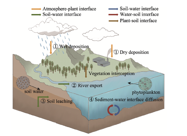
The magnitude of mass flux is closely associated with biogeochemical watershed processes, which can generate a considerable amount of pertinent information. Moreover, both the accuracy and precision of mass flux estimation results directly affects the perception of the ecological environmental status, which in turn affects both the formulation and implementation of river basin management planning. In practical applications, the true value of flux is unknown and can only be estimated. Flux results obtained using different monitoring and estimation methods also differ significantly. However, in existing studies on mass flux associated with biogeochemical watershed interfaces, the application of monitoring and estimation methods lacks uniform criteria or references. Accordingly, this study summarizes and deconstructs results from recent studies on biogeochemical watershed interface processes and compares the advantages, disadvantages and applicability of the monitoring and estimation methods used by these studies. This particular study is intended to be used as a reference for the selection of flux calculation methods.
Key words: flux; basin; monitoring; estimation; biogeochemical cycle
LU Yao , GAO Yang , YANG Tiantian . A review of mass flux monitoring and estimation methods for biogeochemical interface processes in watersheds[J]. Journal of Geographical Sciences, 2020 , 30(6) : 881 -907 . DOI: 10.1007/s11442-020-1760-5
Figure 1 Mass flux associated with biogeochemical watershed interface processes driven by hydrological process (Numbers 1 through 4 correspond to sections 3.1 and 3.4 in this study, respectively. Different colored arrows represent different interface processes.) |
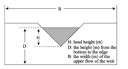
Figure 2 Right-angled triangular weir (Zhu, 2008) |
Table 1 Seven methods for calculating river material flux (A-E are interpolation method, F and G are extrapolation methods) (Webb et al., 1997; Johnes, 2007) |
| No. | Name | Equation | Description | Applicability | References |
|---|---|---|---|---|---|
| A | Interpolation methods | ${\rm{Load}} = {\rm{K}}\left( {\mathop \sum \limits_{{\rm{i}} = 1}^{\rm{n}} \frac{{{{\rm{C}}_{\rm{i}}}}}{{\rm{n}}}} \right)\left( {\mathop \sum \limits_{{\rm{i}} = 1}^{\rm{n}} \frac{{{{\rm{Q}}_{\rm{i}}}}}{{\rm{n}}}} \right)$ | K=conversion factor to take account of period of record Ci =instantaneous concentration associated with individual samples (mg l-1) Qi =instantaneous discharge at time of sampling (m3 s-1) ${{\rm{\bar Q}}_{\rm{r}}}$=mean discharge for period of record (m3 s-1) ${{\rm{\bar Q}}_{\rm{p}}}$=mean discharge for interval between samples (m3 s-1) n=number of samples | Underestimate suspended sediment flux, but are relatively accurate | Webb et al., 1997 |
| B | ${\rm{Load}} = {\rm{K}}\left( {\mathop \sum \limits_{{\rm{i}} = 1}^{\rm{n}} \frac{{{{\rm{C}}_{\rm{i}}}}}{{\rm{n}}}} \right){{\rm{\bar Q}}_{\rm{r}}}$ | Webb et al., 1997 | |||
| C | ${\rm{Load}} = {\rm{K}}\mathop \sum \limits_{{\rm{i}} = 1}^{\rm{n}} \left( {\frac{{{{\rm{C}}_{\rm{i}}}{{\rm{Q}}_{\rm{i}}}}}{{\rm{n}}}} \right)$ | Is suitable for pollutants whose flux is not closely associated to the flow rate | Hao et al., 2012 Wang et al., 2011 | ||
| D | ${\rm{Load}} = {\rm{K}}\mathop \sum \limits_{{\rm{i}} = 1}^{\rm{n}} \left( {{{\rm{C}}_{\rm{i}}}{{{\rm{\bar Q}}}_{\rm{p}}}} \right)$ | Are suitable for pollutants whose flux is closely associated with the flow rate | Hao et al., 2012 | ||
| E | ${\rm{Load}} = \frac{{{\rm{K}}\mathop \sum \nolimits_{{\rm{i}} = 1}^{\rm{n}} \left( {{{\rm{C}}_{\rm{i}}}{{\rm{Q}}_{\rm{i}}}} \right)}}{{\mathop \sum \nolimits_{{\rm{i}} = 1}^{\rm{n}} {{\rm{Q}}_{\rm{i}}}}}{{\rm{\bar Q}}_{\rm{r}}}$ | Zhang et al., 2015 Hao et al., 2012 | |||
| F | Interpolation method: Log-log rating | ${{\rm{C}}_{\rm{i}}} = {\rm{aQ}}_{\rm{i}}^{\rm{b}}$ | $e_i$=log($C_i$)-log($C_{ei}$) Log-log estimate of concentration is multiplied by CF2 to give ‘smeared’ estimate of concentration | The estimation of suspended sediment flux using method F is relatively low | Johnes et al., 2007 |
| G | Interpolation method: Smearing estimate | ${\rm{CF}}2 = \frac{1}{{\rm{n}}}\mathop \sum \limits_{{\rm{i}} = 1}^{\rm{n}} {10^{{{\rm{e}}_{\rm{i}}}}}$ |
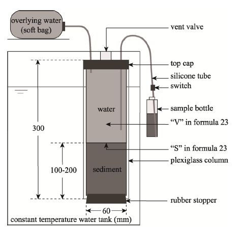
Figure 3 The intact core sediment incubation device (Wang et al., 2018) |
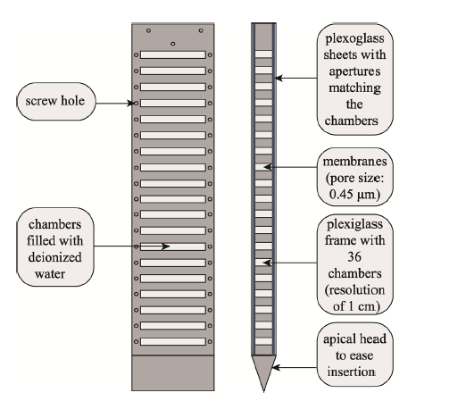
Figure 4 Diagram of a high-resolution peeper device (Yang et al., 2016) |
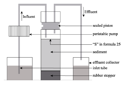
Figure 5 Sketch map of the intact sediment column flow-through system (Rydin, 2000; Xu et al., 2009) |
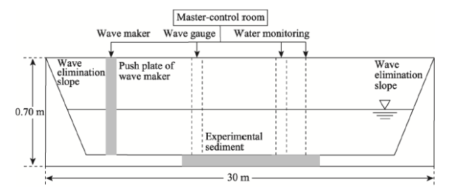
Figure 6 Wave sink (Zhu et al., 2005) |
Table 2 Mass flux monitoring and estimation methods for biogeochemical interface processes in watersheds and their respective advantages and disadvantages |
| Processes | Interface | Methods | Advantages | Disadvantages |
|---|---|---|---|---|
| Wet deposition | Atmosphere-plant-soil interface | Precipitation collection method | Automatically records precipitation; Equipped with refrigeration equipment | ① Requires a stable power supply |
| Ion exchange resin method | Low requirements for sample storage conditions; Can capture cloud deposition | ①High requirements of working temperatures ②Prone to aging effects | ||
| Processes | Interface | Methods | Advantages | Disadvantages |
| Dry deposition | Atmosphere-plant-soil interface | Wet collection method of dust collector | Easy to operate; Low cost | Inconvenient sample transport; Water easily overflows from the dust trap; Prone to evaporate in summer and freeze in winter |
| Model simulation method | No particular need for sensitive sensors; Long-term large-scale deposition flux estimation | Low estimations accuracy | ||
| Soil leaching | Plant-soil-water interface | In-situ plot method | Small workload; Low cost | Typical plots are difficult to select; Not conducive to observing spatial differences |
| Soil tank simulation experimental method | Easy to control experimental conditions and observe experimental results; No need for long-term field observations | Impossible to exclude potential deviations from natural conditions | ||
| Model simulation method | Simulation results are more accurate | Other parameters required | ||
| River export | Plant-soil-water interface | Concentration-flow method | Easy to understand; Easy to calculate | High data intensity requirements; High cost of monitoring |
| Empirical model method | Low data requirements | Poor accuracy | ||
| Mechanistic model method | Good accuracy | A large number of input parameters are required | ||
| Sediment-water interface diffusion | Soil-water interface/water-soil interface | Static culture of the original column | Consideration is given to the consistency between experimental conditions and real environmental conditions | Material concentrations in overlying water cannot be kept constant; Constrained by the sidewall effect |
| Concentration diffusion model of interstitial water | Good accuracy | High data accuracy requirements; Vulnerable to disturbances | ||
| Flow culture of the primary column | Consideration is given to the consistency between experimental conditions and real environmental conditions; Experimental conditions can be kept constant | Complex operation; Constrained by the sidewall effect | ||
| Flume experiment | Consideration is given to the consistency between experimental conditions and real environmental conditions; The sidewall effect is well resolved | Undisturbed sediments are difficult to use as test material |
| [1] |
|
| [2] |
|
| [3] |
|
| [4] |
|
| [5] |
|
| [6] |
|
| [7] |
|
| [8] |
|
| [9] |
|
| [10] |
|
| [11] |
|
| [12] |
|
| [13] |
|
| [14] |
|
| [15] |
|
| [16] |
|
| [17] |
|
| [18] |
|
| [19] |
|
| [20] |
|
| [21] |
|
| [22] |
|
| [23] |
|
| [24] |
|
| [25] |
|
| [26] |
|
| [27] |
|
| [28] |
|
| [29] |
|
| [30] |
|
| [31] |
|
| [32] |
|
| [33] |
|
| [34] |
|
| [35] |
|
| [36] |
|
| [37] |
|
| [38] |
|
| [39] |
|
| [40] |
|
| [41] |
|
| [42] |
|
| [43] |
|
| [44] |
|
| [45] |
|
| [46] |
|
| [47] |
|
| [48] |
|
| [49] |
|
| [50] |
|
| [51] |
|
| [52] |
|
| [53] |
|
| [54] |
|
| [55] |
|
| [56] |
|
| [57] |
|
| [58] |
|
| [59] |
|
| [60] |
|
| [61] |
|
| [62] |
|
| [63] |
|
| [64] |
|
| [65] |
|
| [66] |
|
| [67] |
|
| [68] |
|
| [69] |
|
| [70] |
|
| [71] |
|
| [72] |
|
| [73] |
|
| [74] |
|
| [75] |
|
| [76] |
|
| [77] |
|
| [78] |
|
| [79] |
|
| [80] |
|
| [81] |
|
| [82] |
|
| [83] |
|
| [84] |
|
| [85] |
|
| [86] |
|
| [87] |
|
| [88] |
|
| [89] |
|
| [90] |
|
| [91] |
|
| [92] |
|
| [93] |
|
| [94] |
|
| [95] |
|
| [96] |
|
| [97] |
|
| [98] |
|
| [99] |
|
| [100] |
|
| [101] |
|
| [102] |
|
| [103] |
|
| [104] |
|
| [105] |
|
| [106] |
|
| [107] |
|
| [108] |
|
| [109] |
|
| [110] |
|
| [111] |
|
| [112] |
|
| [113] |
|
| [114] |
|
| [115] |
|
| [116] |
|
| [117] |
|
| [118] |
|
| [119] |
|
| [120] |
|
| [121] |
|
| [122] |
|
| [123] |
|
| [124] |
|
| [125] |
|
| [126] |
|
| [127] |
|
| [128] |
|
| [129] |
|
| [130] |
|
| [131] |
|
| [132] |
|
| [133] |
|
| [134] |
|
| [135] |
|
| [136] |
|
| [137] |
|
| [138] |
|
| [139] |
|
| [140] |
|
| [141] |
|
| [142] |
|
| [143] |
|
| [144] |
|
| [145] |
|
| [146] |
|
| [147] |
|
| [148] |
|
| [149] |
|
| [150] |
|
| [151] |
|
| [152] |
|
| [153] |
|
| [154] |
|
| [155] |
|
| [156] |
|
| [157] |
|
| [158] |
|
| [159] |
|
| [160] |
|
| [161] |
|
| [162] |
|
| [163] |
|
| [164] |
|
| [165] |
|
| [166] |
|
| [167] |
|
| [168] |
|
| [169] |
|
| [170] |
|
/
| 〈 |
|
〉 |