
Journal of Geographical Sciences >
Surplus or deficit? Quantifying the total ecological compensation of Beijing-Tianjin-Hebei Region
|
Yang Wenjie (1990-), PhD Candidate, specialized in resource and environmental economic policy. E-mail: gs_ywj@163.com |
Received date: 2019-03-23
Accepted date: 2019-09-12
Online published: 2020-06-25
Supported by
National Social Science Foundation of China(18BGL173)
National Social Science Foundation of China(16CJY044)
Beijing Social Science Fund Project, China(16LJC009)
Copyright
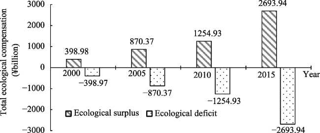
The calculation of ecological compensation and boundary identification of stakeholders represent the key challenges for Beijing-Tianjin-Hebei Region in its implementation of the trans-regional ecological compensation mechanism. Breaking administrative boundaries and spatially coordinating ecological resources helps to restructure an ecological compensation mechanism of the region based on the coordinated development of Beijing, Tianjin and Hebei. According to the estimated ecological assets in the counties of the region in 2000, 2005, 2010 and 2015, a quantitative model for total ecological compensation was built based on ecological assets and county-level economic development. Then, the spatiotemporal distribution characteristics of the total ecological compensation in the region were defined, and the boundaries of ecological surplus and deficit areas were identified. Results indicate: (1) The region’s annual average ecological assets amounted to ¥1379.47 billion; in terms of annual total ecological assets, Hebei ranked first (¥1123.80 billion), followed by Beijing (¥157.46 billion) and Tianjin (¥98.21 billion); and in terms of ecological assets per unit area, Beijing ranked first, Tianjin second and Hebei last. (2) Among ecosystem services, hydrological regulation and climate regulation had the highest annual average value and contributed most to the increase in ecological assets. In 2015, the contribution of water and soil conservation to the total ecological assets decreased to -15.66%, showing the degradation of the function played by different ecosystems. (3) The ecological surplus of the region in four periods of 2000, 2005, 2010 and 2015 were ¥398.98 billion, ¥870.37 billion, ¥1254.93 billion and ¥2693.94 billion respectively, basically offsetting the ecological deficit of each corresponding period, but the urgency for ecological compensation was increased. (4) The ecological surplus and deficit areas showed a great fluctuation in different time periods. Larger time span means more noticeable convergence of deficit areas towards central and eastern areas. Public resources such as education, transportation and medical care in central urban areas should be decentralized to encourage population dispersal, weaken the agglomeration effect of deficit areas and finally achieve the ecological synergy of the region.
YANG Wenjie , GONG Qianwen , ZHANG Xueyan . Surplus or deficit? Quantifying the total ecological compensation of Beijing-Tianjin-Hebei Region[J]. Journal of Geographical Sciences, 2020 , 30(4) : 621 -641 . DOI: 10.1007/s11442-020-1746-3
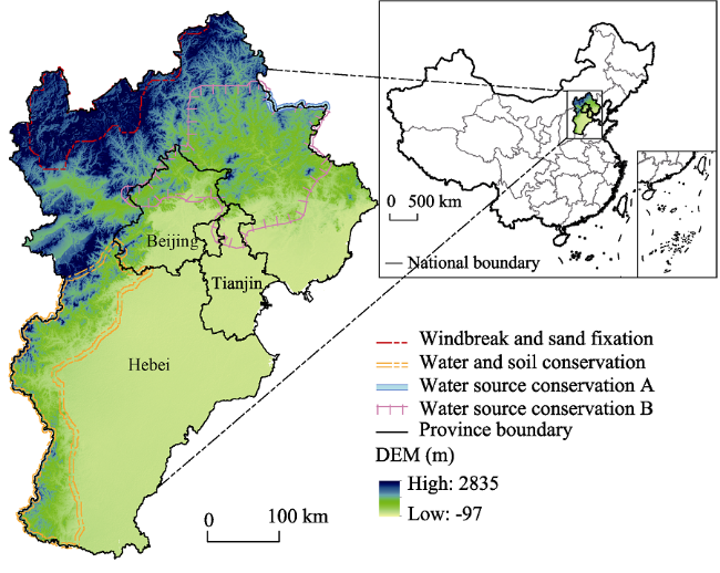
Figure 1 DEM and ecological function zoning of the regionSource: DEM 90 m data and Chinese ecological function zoning data were derived from the Data Center for Resources and Environmental Sciences of CAS. Notes: Windbreak and sand fixation is the ecological function zone at northern foot of the Yinshan Mountain-Hunshandake Sandy Land. Soil conservation is the ecological function zone of the Taihang Mountains. Water source conservation A is the ecological function zone for West Liaohe River source conservation. Water source conservation B is the ecological function zone for Beijing-Tianjin water source conservation. |
Table 1 Unit area ecosystem service value equivalent scale |
| Ecosystem types | Supply service | Regulation service | Support service | Cultural service | ||||||||
|---|---|---|---|---|---|---|---|---|---|---|---|---|
| Primary classification | Secondary classification | FP | RMP | WS | AR | CR | EP | HR | SC | NCM | BD | AL |
| Farmland | Dry land | 0.85 | 0.40 | 0.02 | 0.67 | 0.36 | 0.10 | 0.27 | 1.03 | 0.12 | 0.13 | 0.06 |
| Paddy field | 1.36 | 0.09 | -2.63 | 1.11 | 0.57 | 0.17 | 2.72 | 0.01 | 0.19 | 0.21 | 0.09 | |
| Forest | Woodland | 0.31 | 0.71 | 0.37 | 2.35 | 7.03 | 1.99 | 3.51 | 2.86 | 0.22 | 2.60 | 1.14 |
| Sparse shrubbery | 0.19 | 0.43 | 0.22 | 1.41 | 4.23 | 1.28 | 3.35 | 1.72 | 0.13 | 1.57 | 0.69 | |
| Grassland | High coverage grassland | 0.38 | 0.56 | 0.31 | 1.97 | 5.21 | 1.72 | 3.82 | 2.40 | 0.18 | 2.18 | 0.96 |
| Moderate coverage grassland | 0.22 | 0.33 | 0.18 | 1.14 | 3.02 | 1.00 | 2.21 | 1.39 | 0.11 | 1.27 | 0.56 | |
| Low coverage grassland | 0.10 | 0.14 | 0.08 | 0.51 | 1.34 | 0.44 | 0.98 | 0.62 | 0.05 | 0.56 | 0.25 | |
| Waters | Canal, lake, reservoir | 0.80 | 0.23 | 8.29 | 0.77 | 2.29 | 5.55 | 102.24 | 0.93 | 0.07 | 2.55 | 1.89 |
| Wetland | Mud flat, bottom land, marsh | 0.51 | 0.50 | 2.59 | 1.90 | 3.60 | 3.60 | 24.23 | 2.31 | 0.18 | 7.87 | 4.73 |
| Desert | Sandy land, saline-alkali soil | 0.01 | 0.03 | 0.02 | 0.11 | 0.10 | 0.31 | 0.21 | 0.13 | 0.01 | 0.12 | 0.05 |
| Bare soil, bare rock | 0.00 | 0.00 | 0.00 | 0.02 | 0.00 | 0.10 | 0.03 | 0.02 | 0.00 | 0.02 | 0.01 | |
Notes: FP: food production; RMP: raw material production; WS: water supply; AR: air regulation; CR: climate regulation; EP: environment purification; HR: hydrological regulation; SC: soil conservation; NCM: nutrients cycle maintenance; BD: biodiversity; AL: aesthetic landscape. |
Table 2 Changes in ecological assets of different ecosystem types each period (billion yuan) |
| Ecosystem types | 2000 | 2005 | Growth rate (%) | 2010 | Growth rate (%) | 2015 | Growth rate (%) |
|---|---|---|---|---|---|---|---|
| Farmland | 68.67 | 163.16 | 137.60 | 229.69 | 40.78 | 464.11 | 102.06 |
| Forest | 241.82 | 553.21 | 128.77 | 814.62 | 47.25 | 823.14 | 1.05 |
| Grassland | 101.99 | 235.30 | 130.71 | 357.51 | 51.94 | 423.87 | 18.56 |
| Waters | 77.73 | 171.64 | 120.82 | 253.01 | 47.41 | 259.26 | 2.47 |
| Wetland | 26.31 | 58.73 | 123.22 | 89.54 | 52.46 | 103.37 | 15.45 |
| Desert | 0.12 | 0.28 | 133.33 | 0.42 | 50.00 | 0.39 | -7.14 |
| Total (unchanged price in 2000) | 516.64 | 1182.32 | 128.85 | 1744.79 | 47.57 | 2074.14 | 18.88 |
Notes: Constant price of all data were calculated based on the year 2000. |
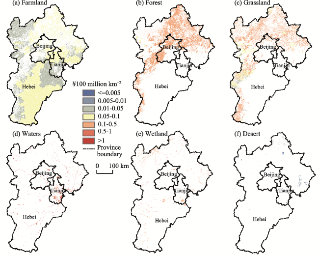
Figure 2 Distribution map of average value of ecological assets for different ecosystem types in 2015 |
Table 3 Changes in the value of regional ecosystem services and their contribution in different periods (¥ billion) |
| Service type | 2000 | 2005 | 2010 | 2015 | ||||
|---|---|---|---|---|---|---|---|---|
| Value | Contribution (%) | Value | Contribution (%) | Value | Contribution (%) | Value | Contribution (%) | |
| Food production | 22.89 | 4.43 | 56.47 | 5.04 | 80.04 | 4.19 | 160.37 | 24.39 |
| Raw material production | 17.29 | 3.35 | 42.16 | 3.74 | 61.48 | 3.43 | 101.10 | 12.03 |
| Water supply | 10.59 | 2.05 | 17.84 | 1.09 | 27.18 | 1.66 | 27.80 | 0.19 |
| Gas regulation | 46.57 | 9.01 | 111.86 | 9.81 | 165.02 | 9.45 | 245.33 | 24.38 |
| Climate regulation | 101.28 | 19.60 | 240.08 | 20.85 | 360.67 | 21.44 | 446.60 | 26.09 |
| Environment purification | 33.71 | 6.52 | 80.71 | 7.06 | 120.52 | 7.08 | 149.73 | 8.87 |
| Hydrological regulation | 139.10 | 26.92 | 283.93 | 21.76 | 426.33 | 25.32 | 422.38 | -1.20 |
| Soil conservation | 77.68 | 15.04 | 187.93 | 16.56 | 262.32 | 13.23 | 210.75 | -15.66 |
| Nutrients cycle maintenance | 5.52 | 1.07 | 13.36 | 1.18 | 19.46 | 1.08 | 32.09 | 3.83 |
| Biodiversity | 42.39 | 8.20 | 101.04 | 8.81 | 151.53 | 8.98 | 189.65 | 11.57 |
| Aesthetic landscape | 19.64 | 3.80 | 46.94 | 4.10 | 70.24 | 4.14 | 88.33 | 5.49 |
| Total (unchanged price in 2000) | 516.64 | 100.00 | 1182.32 | 100.00 | 1744.79 | 100.00 | 2074.14 | 100.00 |
Notes: Constant price of all data were calculated based on the year 2000. |
Figure 3 Total ecological compensation of the region in different periodsNotes: Constant price of all data were calculated based on the year 2000 |
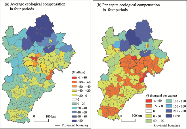
Figure 4 Spatial distribution maps of average ecological compensation among the counties in the regionNotes: Constant price of all data were calculated based on the year 2000. |
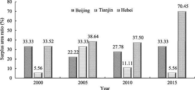
Figure 5 The share of ecological surplus areas at county level in the region in different periods |
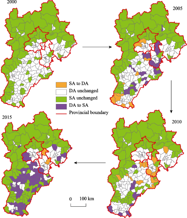
Figure 6 Spatiotemporal change distribution of ecological deficit and surplus areas in the region |
| [1] |
|
| [2] |
|
| [3] |
|
| [4] |
|
| [5] |
|
| [6] |
|
| [7] |
|
| [8] |
|
| [9] |
|
| [10] |
|
| [11] |
|
| [12] |
|
| [13] |
|
| [14] |
|
| [15] |
|
| [16] |
|
| [17] |
|
| [18] |
|
| [19] |
|
| [20] |
|
| [21] |
|
| [22] |
|
| [23] |
|
| [24] |
|
| [25] |
|
| [26] |
|
| [27] |
|
| [28] |
|
| [29] |
|
| [30] |
|
| [31] |
|
| [32] |
|
| [33] |
|
| [34] |
|
| [35] |
|
| [36] |
|
| [37] |
|
| [38] |
|
| [39] |
|
| [40] |
|
| [41] |
|
| [42] |
|
/
| 〈 |
|
〉 |