
Journal of Geographical Sciences >
Spatiotemporal evolution of urban carbon emission performance in China and prediction of future trends
|
Wang Shaojian (1986−), Associate Professor, specialized in urban geography and regional development. E-mail: 1987wangshaojian@163.com |
Received date: 2020-01-06
Accepted date: 2020-03-10
Online published: 2020-07-25
Supported by
Fundamental Research Funds for the Central Universities(19lgzd09)
Guangdong Special Support Program
Pearl River S&T Nova Program of Guangzhou(201806010187)
Copyright
Climate change resulting from CO2 emissions has become an important global environmental issue in recent years. Improving carbon emission performance is one way to reduce carbon emissions. Although carbon emission performance has been discussed at the national and industrial levels, city-level studies are lacking due to the limited availability of statistics on energy consumption. In this study, based on city-level remote sensing data on carbon emissions in China from 1992-2013, we used the slacks-based measure of super-efficiency to evaluate urban carbon emission performance. The traditional Markov probability transfer matrix and spatial Markov probability transfer matrix were constructed to explore the spatiotemporal evolution of urban carbon emission performance in China for the first time and predict long-term trends in carbon emission performance. The results show that urban carbon emission performance in China steadily increased during the study period with some fluctuations. However, the overall level of carbon emission performance remains low, indicating great potential for improvements in energy conservation and emission reduction. The spatial pattern of urban carbon emission performance in China can be described as “high in the south and low in the north,” and significant differences in carbon emission performance were found between cities. The spatial Markov probabilistic transfer matrix results indicate that the transfer of carbon emission performance in Chinese cities is stable, resulting in a “club convergence” phenomenon. Furthermore, neighborhood backgrounds play an important role in the transfer between carbon emission performance types. Based on the prediction of long-term trends in carbon emission performance, carbon emission performance is expected to improve gradually over time. Therefore, China should continue to strengthen research and development aimed at improving urban carbon emission performance and achieving the national energy conservation and emission reduction goals. Meanwhile, neighboring cities with different neighborhood backgrounds should pursue cooperative economic strategies that balance economic growth, energy conservation, and emission reductions to realize low-carbon construction and sustainable development.
WANG Shaojian , GAO Shuang , HUANG Yongyuan , SHI Chenyi . Spatiotemporal evolution of urban carbon emission performance in China and prediction of future trends[J]. Journal of Geographical Sciences, 2020 , 30(5) : 757 -774 . DOI: 10.1007/s11442-020-1754-3
Figure 1 Effects of different factors on urban carbon emission performance from an input-output perspective |
Table 1 System of input-output indicators for carbon emission performance |
| Indicator | Variable | Unit | Mean | Min | Max | S.D. |
|---|---|---|---|---|---|---|
| Input | Fixed-asset investment | 108 yuan | 42.65 | 12.95 | 836.24 | 66.34 |
| Number of employees | 104 person | 220.36 | 0.32 | 1729.55 | 169.70 | |
| Electricity consumption | 104 kwh | 680.87 | 0.25 | 8514.69 | 907.31 | |
| Expected output | GDP | 108 yuan | 103.97 | 2.96 | 1483.55 | 125.46 |
| Non-expected output | CO2 emissions | 104 t | 1665.89 | 0.62 | 20832.94 | 2219.91 |
Table 2 Markov transfer probability matrix (k = 4) |
| t/t+1 | 1 | 2 | 3 | 4 |
|---|---|---|---|---|
| 1 | P11 | P12 | P13 | P14 |
| 2 | P21 | P22 | P23 | P24 |
| 3 | P31 | P32 | P33 | P34 |
| 4 | P41 | P42 | P 43 | P44 |
Table 3 Spatial Markov transfer probability matrix (k = 4) |
| Lag | t/t+1 | 1 | 2 | 3 | 4 |
|---|---|---|---|---|---|
| 1 | 1 | P11|1 | P12|1 | P13|1 | P14|1 |
| 2 | P21|1 | P22|1 | P23|1 | P24|1 | |
| 3 | P31|1 | P32|1 | P33|1 | P34|1 | |
| 4 | P41|1 | P42|1 | P43|1 | P44|1 | |
| 2 | 1 | P11|2 | P12|2 | P13|2 | P14|2 |
| 2 | P21|2 | P22|2 | P23|2 | P24|2 | |
| 3 | P31|2 | P32|2 | P33|2 | P34|2 | |
| 4 | P41|2 | P42|2 | P43|2 | P44|2 | |
| 3 | 1 | P11|3 | P12|3 | P13|3 | P14|3 |
| 2 | P21|3 | P22|3 | P23|3 | P24|3 | |
| 3 | P31|3 | P32|3 | P33|3 | P34|3 | |
| 4 | P41|3 | P42|3 | P43|3 | P44|3 | |
| 4 | 1 | P11|4 | P12|4 | P13|4 | P14|4 |
| 2 | P21|4 | P22|4 | P23|4 | P24|4 | |
| 3 | P31|4 | P32|4 | P33|4 | P34|4 | |
| 4 | P41|4 | P42|4 | P43|4 | P44|4 |
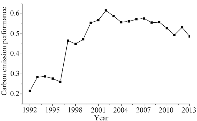
Figure 2 Evolution in urban carbon emission performance from 1992-2013 |
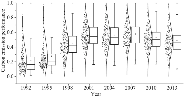
Figure 3 Box plot of urban carbon emission performance in Chinese cities from 1992 to 2013 |
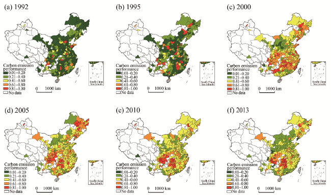
Figure 4 Spatial distributions of urban carbon emission performance in Chinese cities from 1992-2013 |
Table 4 Markov matrix of city-level carbon emission performance types from 1992-2013 |
| t/t+1 | n | 1 | 2 | 3 | 4 |
|---|---|---|---|---|---|
| 1 | 1514 | 0.7437 | 0.1777 | 0.0575 | 0.0211 |
| 2 | 1457 | 0.1030 | 0.6603 | 0.1929 | 0.0439 |
| 3 | 1472 | 0.0177 | 0.1793 | 0.6372 | 0.1658 |
| 4 | 1500 | 0.0133 | 0.0253 | 0.1600 | 0.8013 |
Table 5 Spatial Markov matrix of city-level carbon emission performance in China from 1992-2013 |
| Lag | t/t+1 | n | 1 | 2 | 3 | 4 |
|---|---|---|---|---|---|---|
| 1 | 1 | 807 | 0.7720 | 0.1437 | 0.0595 | 0.0248 |
| 2 | 313 | 0.1565 | 0.6006 | 0.1821 | 0.0607 | |
| 3 | 206 | 0.0388 | 0.2330 | 0.5631 | 0.1650 | |
| 4 | 176 | 0.0341 | 0.0455 | 0.1364 | 0.7841 | |
| 2 | 1 | 470 | 0.7319 | 0.2000 | 0.0553 | 0.0128 |
| 2 | 436 | 0.1124 | 0.6651 | 0.1789 | 0.0436 | |
| 3 | 321 | 0.0218 | 0.2274 | 0.5919 | 0.1589 | |
| 4 | 256 | 0.0430 | 0.0313 | 0.1953 | 0.7305 | |
| 3 | 1 | 182 | 0.6923 | 0.2253 | 0.0495 | 0.0330 |
| 2 | 440 | 0.0750 | 0.6841 | 0.2045 | 0.0364 | |
| 3 | 475 | 0.0147 | 0.1537 | 0.6505 | 0.1811 | |
| 4 | 371 | 0.0054 | 0.0296 | 0.2075 | 0.7574 | |
| 4 | 1 | 55 | 0.6000 | 0.3273 | 0.0727 | 0.0000 |
| 2 | 268 | 0.0709 | 0.6828 | 0.2090 | 0.0373 | |
| 3 | 470 | 0.0085 | 0.1489 | 0.6872 | 0.1553 | |
| 4 | 697 | 0.0014 | 0.0158 | 0.1277 | 0.8551 |
Table 6 Predicted evolution in carbon emission performance in Chinese cities |
| State type | 1 | 2 | 3 | 4 | ||
|---|---|---|---|---|---|---|
| Ignoring spatial lag | Initial state | 0.1484 | 0.3534 | 0.3004 | 0.1979 | |
| Ultimate state | 0.1377 | 0.2512 | 0.2948 | 0.3162 | ||
| Considering spatial lag | Ultimate state | 1 | 0.2521 | 0.2524 | 0.2242 | 0.2713 |
| 2 | 0.1908 | 0.3184 | 0.2708 | 0.2201 | ||
| 3 | 0.0851 | 0.2585 | 0.3471 | 0.3093 | ||
| 4 | 0.0477 | 0.2220 | 0.3249 | 0.4054 | ||
| [1] |
|
| [2] |
|
| [3] |
|
| [4] |
|
| [5] |
|
| [6] |
IEA, 2012. World Energy Outlook 2012. Paris:International Energy Agency (IEA).
|
| [7] |
|
| [8] |
|
| [9] |
|
| [10] |
|
| [11] |
|
| [12] |
|
| [13] |
|
| [14] |
|
| [15] |
|
| [16] |
|
| [17] |
|
| [18] |
|
| [19] |
|
| [20] |
|
| [21] |
|
| [22] |
|
| [23] |
|
| [24] |
|
| [25] |
|
| [26] |
|
| [27] |
|
| [28] |
|
| [29] |
|
| [30] |
|
| [31] |
|
| [32] |
|
| [33] |
|
| [34] |
|
| [35] |
|
| [36] |
|
| [37] |
|
| [38] |
|
| [39] |
|
| [40] |
|
| [41] |
|
| [42] |
|
| [43] |
|
| [44] |
|
| [45] |
|
| [46] |
|
| [47] |
|
| [48] |
|
| [49] |
|
| [50] |
|
| [51] |
|
| [52] |
|
| [53] |
|
| [54] |
|
| [55] |
|
/
| 〈 |
|
〉 |
