
Journal of Geographical Sciences >
Exploring global food security pattern from the perspective of spatio-temporal evolution
|
Cai Jianming (1961-), Professor, specialized in urban and rural sustainable development. E-mail: caijm@igsnrr.ac.cn |
Received date: 2019-08-02
Accepted date: 2019-10-30
Online published: 2020-04-21
Supported by
National Natural Science Foundation of China(No.71734001)
Copyright
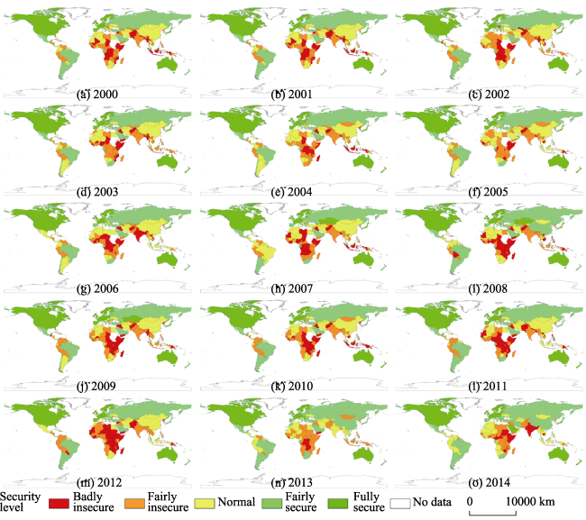
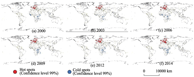
Food security is the primary prerequisite for achieving other Millennium Development Goals (MDGs). Given that the MDG of “halving the proportion of hungers by 2015” was not realized as scheduled, it will be more pressing and challenging to reach the goal of zero hunger by 2030. So there is high urgency to find the pattern and mechanism of global food security from the perspective of spatio-temporal evolution. In this paper, based on the analysis of database by using a multi-index evaluation method and radar map area model, the global food security level for 172 countries from 2000 to 2014 were assessed; and then spatial autocorrelation analysis was conducted to depict the spatial patterns and changing characteristics of global food security; then, multi-nonlinear regression methods were employed to identify the factors affecting the food security patterns. The results show: 1) The global food security pattern can be summarized as “high-high aggregation, low-low aggregation”. The most secure countries are mainly distributed in Western Europe, North America, Oceania and parts of East Asia. The least secure countries are mainly distributed in sub-Saharan Africa, South Asia and West Asia, and parts of Southeast Asia. 2) Europe and sub-Saharan Africa are hot and cold spots of the global food security pattern respectively, while in non-aggregation areas, Haiti, North Korea, Tajikistan and Afghanistan have long-historical food insecurity problems. 3) The pattern of global food security is generally stable, but the internal fluctuations in the extremely insecure groups were significant. The countries with the highest food insecurity are also the countries with the most fluctuated levels of food security. 4) The annual average temperature, per capita GDP, proportion of people accessible to clean water, political stability and non-violence levels are the main factors influencing the global food security pattern. Research shows that the status of global food security has improved since the year 2000, yet there are still many challenges such as unstable global food security and acute regional food security issues. It will be difficult to understand these differences from a single factor, especially the annual average temperature and annual precipitation. The abnormal performance of the above factors indicates that appropriate natural conditions alone do not absolutely guarantee food security,while the levels of agricultural development, the purchasing power of residents, regional accessibility, as well as political and economic stability have more direct influence.
CAI Jianming , MA Enpu , LIN Jing , LIAO Liuwen , HAN Yan . Exploring global food security pattern from the perspective of spatio-temporal evolution[J]. Journal of Geographical Sciences, 2020 , 30(2) : 179 -196 . DOI: 10.1007/s11442-020-1722-y
Table 1 Evaluation index system and measurement methods of food security |
| Overall index | First layer factors | Second layer indicators | +/- influence | Measurement methods |
|---|---|---|---|---|
| Food security index | Food supply | X1: per capita food production (kg/person) | +(1) | X1 = total grain production/total population |
| X2: per capita protein supply (g/person*day) | + | X2 = supply of food protein/total population * days of the year | ||
| X3: per capita animal protein supply (g/person*day) | + | X3 = animal protein supply/total population * days of the year | ||
| X4: rate of dietary energy supply (%) | + | X4 = population with daily dietary energy greater than 2320 kcal(2)/total population | ||
| Food access | X5: food deficiency (kcal/person/day) | - | X5 = 2320 - daily per capita dietary energy taken by malnourished populations | |
| X6: per capita GDP (2011- dollar value) | + | X6 = gross domestic product converted by purchasing power parity/total population | ||
| Food utilization | X7: the proportion of short children under 5 (%) | - | X7 = number of short children under 5/number of children under 5 | |
| X8: the proportion of wasted children under 5 (%) | - | X8 = number of wasted children under 5/number of children under 5 | ||
| X9: proportion of population with access to clean water ( % ) | + | X9 = population with clean water/total population | ||
| Economic and political stability | X10: variability in food production per capita | - | X10 = standard deviation of per capita food production/average of per capita food production | |
| X11: variability of food supply per capita(kcal/person/day) | - | X11 = standard deviation of per capita food supply | ||
| X12: political stability and non-violence level | + | X12: World Governance Indicators Developed by the World Bank (WGI)(3) |
Note: (1) The “+” indicates the positive influence, meaning the greater the value, the higher the food security level, while the “-” indicates that the negative influence. (2) 2320 kcal is the minimum daily dietary energy for adults. (3) Political stability and non-violence level is one of the six indicators of the World Governance Indicators (WGI) system. It was first proposed by Kaufman et al. in 1999 and used to measure the perceptions of political stability, political violence and terrorism. |
Table 2 The selection of influencing factors of food security and data sources |
| Influencing factors | Methods and data | Data resource websites |
|---|---|---|
| Z1: per capita arable land area (ha/person) | Z1 = arable land area/total population | http://www.fao.org/faostat/en/ |
| Z2: per capita renewable water resources (m3/person) | Z2 = renewable water resources/total population | renewable water resource:http://chartsbin.com/view/1469;population:http://www.fao.org/faostat/en/ |
| Z3: annual precipitation (mm) | Z3: provided by the climate research unit at the University of East Anglia | https://crudata.uea.ac.uk/cru/data/hrg/cru_ts_3.23/crucy.1506241137.v3.23/countries/pre/ |
| Z4: annual average temperature (℃) | Z4: provided by the climate research unit at the University of East Anglia | https://crudata.uea.ac.uk/cru/data/hrg/cru_ts_3.23/crucy.1506241137.v3.23/countries/tmp/ |
| Z5: coordination degree of land and water | Z5 = renewable water/arable land area | renewable water resource:http://chartsbin.com/view/1469;arable land area:http://www.fao.org/faostat/en/ |
| Z6: chemical fertilizer applied per unit land area (kg/ha) | Z6 = applied chemical fertilizers/arable land area | http://www.fao.org/faostat/en/ |
| Z7: CO2 emissions (kt) | Z7: from the National Greenhouse Gas Emission Dataset of the World Resources Institute. This dataset is a combination of data from Oak Ridge National Laboratory, FAO, International Energy Agency, World Bank, and Environmental Protection Agency. | http://datasets.wri.org/dataset/cait-country |
| Z8: per capita GDP (dollar value in 2011) | Z8 = GDP (dollar value in 2011)/total population | http://www.fao.org/faostat/en/ |
| Z9: the proportion of the population with access to clean water (%) | Z9 = population with access to clean water/total population | http://www.fao.org/faostat/en/ |
| Z10: political stability and non-violence level | Z10: World Governance Indicators Developed by the World Bank | https://datacatalog.worldbank.org/dataset/worldwide-governance-indicators |
Table 3 Weight of each second layer variable |
| First layer indicators | Food supply | Food accessibility | Food utilization | Stability of the economic and political system | ||||||||
|---|---|---|---|---|---|---|---|---|---|---|---|---|
| Second layer variables | X1 | X2 | X3 | X4 | X5 | X6 | X7 | X8 | X9 | X10 | X11 | X12 |
| Weight | 0.21 | 0.28 | 0.33 | 0.18 | 0.51 | 0.49 | 0.39 | 0.31 | 0.3 | 0.27 | 0.31 | 0.42 |
Note: The definition of each second layer variable is shown in Table 1. |
Figure 1 Changes of the global food security pattern by country from 2000 to 2014 |
Table 4 Moran’s I, z-score and P-value of the food security index from 2000 to 2014 |
| Year | 2000 | 2001 | 2002 | 2003 | 2004 | 2005 | 2006 | 2007 | 2008 | 2009 | 2010 | 2011 | 2012 | 2013 | 2014 |
|---|---|---|---|---|---|---|---|---|---|---|---|---|---|---|---|
| Moran's I | 0.22 | 0.22 | 0.22 | 0.23 | 0.24 | 0.25 | 0.28 | 0.27 | 0.28 | 0.26 | 0.29 | 0.25 | 0.27 | 0.24 | 0.27 |
| z-score | 14.00 | 13.84 | 13.71 | 14.40 | 15.14 | 15.39 | 17.12 | 16.51 | 17.69 | 16.44 | 18.27 | 15.44 | 16.68 | 15.04 | 17.04 |
| P-score | 0 | 0 | 0 | 0 | 0 | 0 | 0 | 0 | 0 | 0 | 0 | 0 | 0 | 0 | 0 |
Figure 2 Hot and cold spots of the global food security pattern from 2000 to 2014 |
Table 5 Multi-linear regression equations served as control |
| Year | Multi-linear regression equations | R2 | F | Sig. |
|---|---|---|---|---|
| 2002 | FSI=0.26-0.14Z4+0.60Z8+0.42Z9+0.39Z10 | 0.78 | 114.45 | 0.00 |
| 2003 | FSI=0.22-0.19Z4+0.61Z8+0.49Z9+0.37Z10 | 0.79 | 118.01 | 0.00 |
| 2004 | FSI=0.19-0.19Z4+0.56Z8+0.52Z9+0.39Z10 | 0.78 | 110.60 | 0.00 |
| 2005 | FSI=0.06-0.17Z4+0.51Z8+0.62Z9+0.43Z10 | 0.79 | 117.77 | 0.00 |
| 2006 | FSI=0.31+0.14Z3-0.32Z4+0.71Z8+0.43Z9+0.33Z10 | 0.83 | 124.08 | 0.00 |
| 2007 | FSI=0.20-0.17Z4-0.36Z6+0.70Z8+0.55Z9+0.34Z10 | 0.83 | 121.30 | 0.00 |
| 2008 | FSI=0.32-0.24Z4+0.68Z8+0.47Z9+0.28Z10 | 0.82 | 147.35 | 0.00 |
| 2009 | FSI=0.31+0.11Z3-0.24Z4-0.18Z6+0.76Z8+0.44Z9+0.28Z10 | 0.83 | 102.51 | 0.00 |
| 2010 | FSI=0.26-0.16Z4-0.45Z6+0.86Z8+0.48Z9+0.24Z10 | 0.83 | 124.83 | 0.00 |
| 2011 | FSI=0.009-0.10Z4-0.64Z6+0.82Z8+0.61Z9+0.36Z10 | 0.86 | 153.29 | 0.00 |
| 2012 | FSI=0.23-0.10Z4-0.59Z6+0.83Z8+0.40Z9+0.31Z10 | 0.86 | 152.71 | 0.00 |
| 2013 | FSI=0.28-0.10Z4+0.35Z8+0.31Z9+0.25Z10 | 0.69 | 70.32 | 0.00 |
| 2014 | FSI=0.25-0.12Z4+0.39Z8+0.36Z9+0.28Z10 | 0.72 | 80.87 | 0.00 |
Table 6 Transformation equations |
| Year | Transformation equations | R2 | F | Sig. |
|---|---|---|---|---|
| 2002 | FSI=-0.24+0.09T4+0.57T8+0.30T9+0.29T10 | 0.83 | 160.09 | 0.00 |
| 2003 | FSI=-0.23+0.10T4+0.55T8+0.35T9+0.30T10 | 0.83 | 157.89 | 0.00 |
| 2004 | FSI=-0.28+0.11T4+0.54T8+0.37T9+0.29T10 | 0.82 | 141.20 | 0.00 |
| 2005 | FSI=-0.23+0.06T4+0.47T8+0.42T9+0.33T10 | 0.82 | 146.46 | 0.00 |
| 2006 | FSI=-0.23-0.04T3+0.16T4+0.56T8+0.34T9+0.25T10 | 0.88 | 185.76 | 0.00 |
| 2007 | FSI=-0.22+0.14T4-0.03T6+0.53T8+0.37T9+0.28T10 | 0.84 | 129.99 | 0.00 |
| 2008 | FSI=0.20T4+0.64T8-0.03T9+0.28T10 | 0.85 | 186.05 | 0.00 |
| 2009 | FSI=-0.31+0.04T3+0.16T4-0.02T6+0.59T8+0.28T9+0.30T10 | 0.86 | 128.65 | 0.00 |
| 2010 | FSI=-0.29+0.15T4+0.04T6+0.60T8+0.30T9+0.23T10 | 0.86 | 160.09 | 0.00 |
| 2011 | FSI=-0.22+0.08T4-0.06T6+0.55T8+0.35T9+0.34T10 | 0.85 | 147.59 | 0.00 |
| 2012 | FSI=-0.24+0.10T4-0.001T6+0.60T8+0.26T9+0.33T10 | 0.87 | 162.64 | 0.00 |
| 2013 | FSI=-0.23+0.10T4+0.37T8+0.46T9+0.39T10 | 0.72 | 81.11 | 0.00 |
| 2014 | FSI=-0.24+0.09T4+0.52T8+0.34T9+0.37T10 | 0.77 | 106.88 | 0.00 |
Table 7 Multi-nonlinear regression equations |
| Year | Multi-nonlinear regression equations |
|---|---|
| 2002 | FSI=0.30+0.27Z43-0.41Z42+0.12Z4-1.20Z82+1.52Z8+1.85Z93-2.83Z92+1.35Z9+0.20Z102+0.02Z10 |
| 2003 | FSI=0.31-0.06Z4-1.16Z82+1.47Z8+2.04Z93-2.98Z92+1.31Z9+0.19Z102+0.05Z10 |
| 2004 | FSI=0.28+0.03Z42-0.09Z4+0.25Z83-1.42Z82+1.47Z8+2.19Z93-3.32Z92+1.56Z9+0.11Z103+0.01Z102+0.12Z10 |
| 2005 | FSI=-0.06-0.04Z4-1.01Z82+1.26Z8+3.38Z93-5.54Z92+2.91Z9+0.20Z102+0.27Z10 |
| 2006 | FSI=0.34-0.13Z33+0.18Z32-0.05Z3-0.11Z4-1.18Z82+1.53Z8+2.65Z93-3.95Z92+1.7Z9+0.26Z103-0.17Z102+0.13Z10 |
| 2007 | FSI=0.39-0.09Z4-0.35Z63+0.49Z62-0.15Z6-0.96Z82+1.28Z8+2.40Z93-3.51Z92+1.50Z9+0.22Z102-0.01Z10 |
| 2008 | FSI=0.54-0.14Z4-1.22Z82+1.61Z8+0.30Z92-0.13Z9+0.21Z103-0.08Z102+0.11Z10 |
| 2009 | FSI=0.39+0.12Z33-0.17Z32+0.06Z3-0.11Z4-0.14Z63+0.20Z62-0.08Z6-1.14Z82+1.47Z8+2.13Z93-3.26Z92+1.46Z9 +0.26Z103-0.11Z102+0.10Z10 |
| 2010 | FSI=0.38+0.02Z42-0.12Z4+0.82Z63-1.07Z62+0.26Z6-1.18Z82+1.52Z8+2.47Z93-3.79Z92+1.69Z9+0.24Z103 -0.14Z102+0.10Z10 |
| 2011 | FSI=-0.02-0.05Z4-3.32Z63+3.91Z62-0.61Z6-1.13Z82+1.45Z8+3.10Z93-5.10Z92+2.62Z9+0.45Z103-0.56Z102+0.47Z10 |
| 2012 | FSI=0.35-0.06Z4-0.06Z63+0.07Z62-0.01Z6-1.03Z82+1.39Z8+1.96Z93-3.01Z92+1.34Z9+0.33Z103-0.27Z102+0.23Z10 |
| 2013 | FSI=0.46-0.04Z4+0.32Z83-0.77Z82+0.63Z8+1.69Z93-2.21Z92+0.68Z9+0.29Z103-0.30Z102+0.24Z10 |
| 2014 | FSI=0.49-0.04Z4+0.97Z83-1.90Z82+1.24Z8+1.33Z93-1.70Z92+0.49Z9+0.29Z102-0.09Z10 |
Table 8 Influence coefficient of each factor |
| Year | Annual precipitation | Annual average temperature | Chemical fertilizer applied per unit land area | Per capita GDP | Proportion of the population with access to clean water | Political stability and non-violence level |
|---|---|---|---|---|---|---|
| 2002 | - | -0.0216 | - | 0.3192 | 0.372 | 0.2262 |
| 2003 | - | -0.057 | - | 0.319 | 0.378 | 0.243 |
| 2004 | - | -0.0682 | - | 0.297 | 0.4366 | 0.2436 |
| 2005 | - | -0.0354 | - | 0.2538 | 0.7518 | 0.4713 |
| 2006 | -0.0104 | -0.1104 | - | 0.3472 | 0.3978 | 0.22 |
| 2007 | - | -0.0924 | -0.0087 | 0.318 | 0.3885 | 0.2128 |
| 2008 | - | -0.138 | - | 0.384 | 0.1689 | 0.2324 |
| 2009 | 0.0048 | -0.1056 | -0.0066 | 0.3245 | 0.3276 | 0.252 |
| 2010 | - | -0.1005 | 0.012 | 0.336 | 0.363 | 0.1955 |
| 2011 | - | -0.10 | -0.64 | 0.82 | 0.61 | 0.36 |
| 2012 | - | -0.056 | -0.00029 | 0.354 | 0.2886 | 0.2871 |
| 2013 | - | -0.038 | - | 0.185 | 0.161 | 0.2379 |
| 2014 | - | -0.0378 | - | 0.312 | 0.1224 | 0.2035 |
Note:“-” means that the influencing factors did not appear in the regression equation for that year. |
| [1] |
|
| [2] |
|
| [3] |
|
| [4] |
|
| [5] |
Food and Agriculture Organization of the United Nations, 2002. The State of Food Insecurity in the World 2001. Rome, Italy: Food and Agriculture Organizationof the United Nations.
|
| [6] |
Food and Agriculture Organization of the United Nations, United Nations Children’s Fund, World Food Programme et al., 2017. The State of Food Security and Nutrition in the World 2017: Enhancing Resilience and Promoting Peace and Food Security. Rome, Italy: Food and Agriculture Organization of the United Nations, 4.
|
| [7] |
Future Earth Interim Secretariat (FEIS), 2013. Future Earth Initial Design. Paris: International Council for Science.
|
| [8] |
Future Earth Interim Secretariat (FEIS), 2014. Future Earth 2025 Vision. Paris: International Council for Science.
|
| [9] |
IPCC Working Group III, 2007. Intergovernmental Panel on Climate Change Special Report on Emissions Scenarios. Geneva, Switzerland: Intergovernmental Panel on Climate Change.
|
| [10] |
|
| [11] |
|
| [12] |
|
| [13] |
|
| [14] |
|
| [15] |
|
| [16] |
|
| [17] |
|
| [18] |
|
| [19] |
|
| [20] |
|
| [21] |
|
| [22] |
|
| [23] |
|
| [24] |
|
| [25] |
|
/
| 〈 |
|
〉 |