Research Articles

Exploring spatial-temporal change and gravity center movement of construction land in the Chang-Zhu-Tan urban agglomeration

  • LI Zhuo 1, 2 ,
  • JIANG Weiguo , 1, 2, * ,
  • WANG Wenjie 3 ,
  • LEI Xuan 4 ,
  • DENG Yue 1, 2
Expand
  • 1. State Key Laboratory of Remote Sensing Science, Faculty of Geographical Science, Beijing Normal University, Beijing 100875, China
  • 2. Key Laboratory of Environmental Change and Natural Disaster of Ministry of Education, Faculty of Geographical Science, Beijing Normal University, Beijing 100875, China
  • 3. Chinese Research Academy of Environmental Sciences, Beijing 100012, China
  • 4. Tianjin University Research Institute of Urban Planning, Tianjin 300073, China
*Jiang Weiguo (1976-), PhD and Professor, E-mail:

Li Zhuo (1996-), PhD, specialized in urban wetland and urban ecology. E-mail: lizhuo@mail.bnu.edu.cn

Received date: 2018-09-04

  Accepted date: 2018-12-07

  Online published: 2019-12-13

Supported by

National Natural Science Foundation of China(No.41571077)

National Key Research and Development Program of China(No.2016YFC0503002)

Copyright

Copyright reserved © 2019. Office of Journal of Geographical Sciences All articles published represent the opinions of the authors, and do not reflect the official policy of the Chinese Medical Association or the Editorial Board, unless this is clearly specified.

Abstract

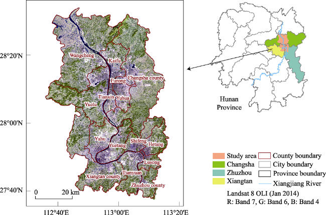
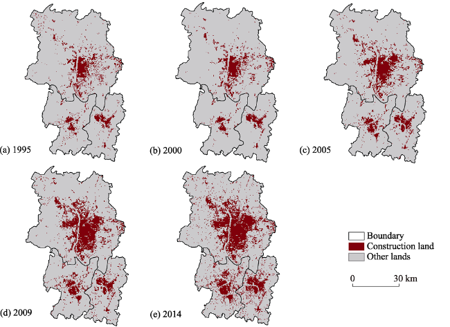
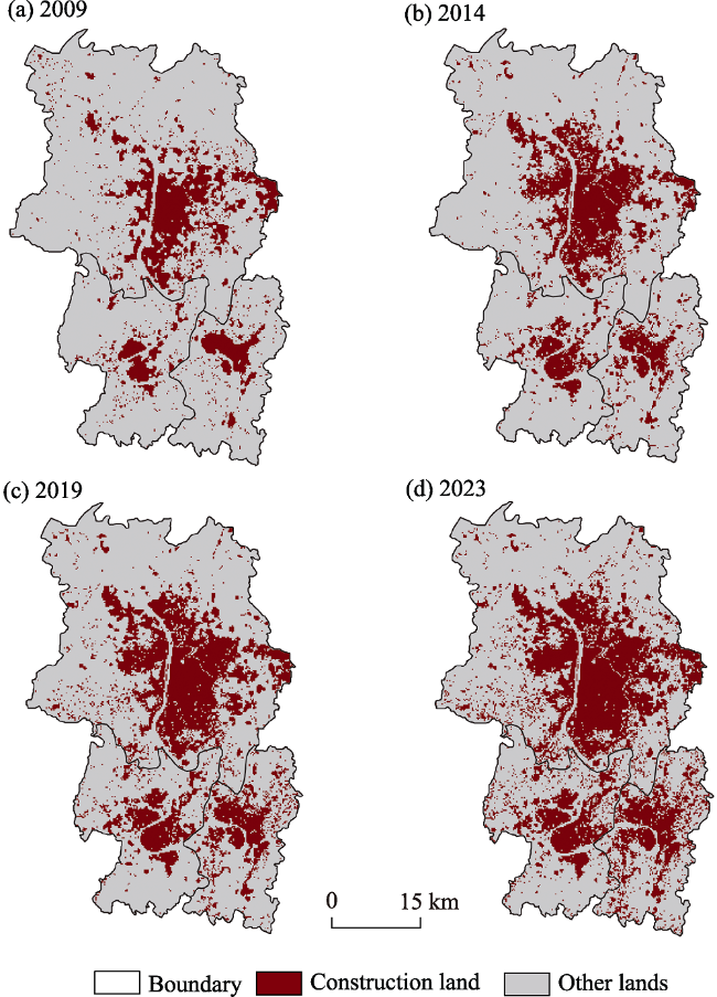
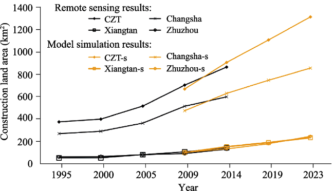
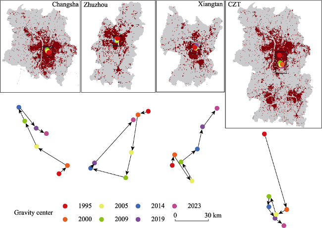
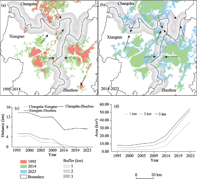
Urban agglomeration is caused by the continuous acceleration of the urbanization process in China. Studying the expansion of construction land can not only know the changes and development of urban agglomeration in time, but also obtain the great significance of the future management. In this study, taking Changsha-Zhuzhou-Xiangtan (Chang-Zhu-Tan) urban agglomeration in Hunan province as a study area, Landsat images from 1995 to 2014 and Autologistic-CLUE-S model simulation data were used. Moreover, several factors including gravity center, direction, distance and landscape index were considered in the analysis of the expansion. The results revealed that the construction area increased by 132.18%, from 372.28 km 2 in 1995 to 864.37 km 2 in 2014. And it might even reach 1327.23 km 2 in 2023. Before 2014, three cities had their own respective and discrete development directions. However, because of the integration policy implementation in 2008, the Chang-Zhu-Tan began to gather, the gravity center moved southward after 2014, and the distance between cities decreased, which was in line with the development plan of urban expansion. The research methods and results were relatively reliable, and these results could provide some reference for the future land use planning and spatial allocation in the urbanization process of Chang-Zhu-Tan urban agglomeration.

Cite this article

LI Zhuo , JIANG Weiguo , WANG Wenjie , LEI Xuan , DENG Yue . Exploring spatial-temporal change and gravity center movement of construction land in the Chang-Zhu-Tan urban agglomeration[J]. Journal of Geographical Sciences, 2019 , 29(8) : 1363 -1380 . DOI: 10.1007/s11442-019-1664-5

1 Introduction

In the past few decades, urbanization has profoundly changed the world and more than half the world’s population now live in cities (Han et al., 2016). Since China is a developing country with a large population, the scale of urbanization is expanding, and its economy and society is experiencing unprecedented rapid development (Deng and Huang, 2004; Chen et al., 2016). By 2016, 54% of Chinese people lived in cities (Zeng et al., 2017). Rapid urbanization is the main driving force of urban land growth (Yu et al., 2014). Moreover, now and in the next few decades, the spatial expansion of construction land will become the main feature of land-use change (Chen et al., 2016). The study of the spatial-temporal characteristics of construction land expansion will further deepen understanding the nature of the urbanization.
A growing amount of literature has documented various methods to study rapid urban expansion (Wei, 2017). Remote sensing data and GIS spatial analysis were used to study the spatial expansion and external morphological evolution of urban or urban agglomeration (Sun and Zhao, 2018; Xu et al., 2018; Yang et al., 2018). Land cover pattern on Landsat satellite images and LUCC were used to study land surface temperature and ecosystem services (Zhou et al., 2011; Wang et al., 2018). In addition, the landscape metrics also could be used to study urbanization and analyze the spatial-temporal pattern of urban sprawl (Seto and Fragkias, 2005; Lv et al., 2012; Zeng et al., 2012). Recently, urban growth models were widely used to simulate the future development of the cities, such as logistic regression, the SLEUTH model, the spatial regression model, and the CLUE-S model (Silva and Clarke, 2002; Rafiee et al., 2009; Puertas et al., 2014; Zeng et al., 2015; Jiang et al., 2017; Vasenev et al., 2018). The Autologistic-CLUE-S model was used in this research to simulate the future development. The CLUE-S model was developed by Verburg et al. on the basis of CLUE model (Veldkamp and Fresco, 1996; Verburg et al., 2002). Many researchers used CLUE-S model to simulate land use change in different scales, including counties, river basins, countries, etc., and obtained relatively good simulation results (Verburg et al., 2006; Castella et al., 2007; Lourdes et al., 2011; Price et al., 2015). It was not difficult to find that this model was widely applied by many scholars because of its wide applicability and openness. And the significance of adding Autologistic was that it could quantitatively analyze the correlation between land use distribution pattern and environmental factors, and also considered the spatial autocorrelation of data.
In the near term, remote sensing, land use, urban growth model were the main methods to study urbanization (Wu et al., 2011; Liu and Chen, 2017; Wang et al., 2018). Also, the gravity center of the construction land area could be used as a method to analyze urban expansion. Gradually, scholars have integrated the GIS spatial analysis method with the gravity center. According to the current research situation, the gravity center was mainly used in economics, population, energy and other fields, and it was also used to study the changes in energy production and consumption centers (Zhang et al., 2012; Wang et al., 2014). The location and movement of the environmental pollution emission gravity center were important indicators that reflected the spatial distribution and change of environmental pollution. And air pollution emissions and economic gravity center were positive correlations (Zhao et al., 2010; Hu et al., 2012). Some researchers calculated the gravity center of consumption and economy in Xinjiang from 1965 to 2009 and obtained the conclusion that the two gravity centers both moved to northeast (Fu et al., 2011). Through the calculation method of gravity center, urban ecological land center was obtained. On this basis, the spatial dynamics of ecological land in Shenzhen City was revealed, and the influencing factors were also analyzed (Peng et al., 2017).
Urban agglomeration is a product of urbanization and is gradually replacing the single city and becomes a new regional economic growth pole with unique advantages. The research methods for urban agglomerations are varied. Also, the researches on gravity center of urban agglomeration land were new research points, but this was seldom mentioned. Beijing-Tianjin-Hebei (Jing-Jin-Ji) urban agglomeration is becoming an important core area in the economy, science and technology, and culture in north China. The gravity center method was used to study the spatial changes and hotspot regions in land use of the core area of Jing-Jin-Ji and it was found that cultivated land area decreased and built-up land grew rapidly (Li et al., 2017). It is important for the urban agglomeration of the Yangtze River Delta to the regional development in China. In this urban agglomeration, the northwestern cities developed with greater speed and larger size than the southern cities, which promoted the urban agglomeration gravity to move toward the northwest (Chen et al., 2007). In the Changsha-Zhuzhou-Xiangtan (Chang-Zhu-Tan) urban agglomeration, the regional population, GDP and the secondary industry center moved to the northwest, and the tertiary industrial and consumer focus shifted to the northeast (Tang and Chen, 2011). The gravity center method was used in this article to analyze the expansion of construction area. So, the research methods of this article were innovative to certain degree.
Chang-Zhu-Tan was chosen as the study area, and the research on the expansion of Chang-Zhu-Tan was based on remote sensing, GIS technology, gravity center, direction, distance and landscape index. Therefore, the specific objectives were (1) to analyze the spatial-temporal change of construction area from 1995 to 2023, (2) to explore the previous change rule of construction area from 1995 to 2014, and (3) to forecast the development direction of construction area in 2019 and 2023.

2 Materials and methods

2.1 Study area

The study area is the core economic area of the Chang-Zhu-Tan urban agglomeration, located in the northeast part of Hunan Province, China, lying between 112°38°-113°17°E and 27°37°-28°33°N (Figure 1). Xiangjiang River, one of the most important tributaries of the Yangtze River, runs through this region from north to south. The geomorphology mainly consists of hills, low-lying land, and plains. This area belongs to the subtropical monsoon climate, and the mean annual temperature fluctuates between 16℃ and 18℃ and the mean annual precipitation is only about 1390 mm (Quan et al., 2013; Jiang et al., 2015). The Chang-Zhu-Tan is an important economic tie which connects the northern and southern cities together. In this region, the roads and railways are well developed, and the traffic conditions in urban agglomeration are superior. In 2007, the National Development and Reform Commission of China designated the Chang-Zhu-Tan as the fourth National Demonstration Area where economic development should be implemented in harmony with resource-saving and environment-friendly land-use practices.
Figure 1 Location of the study area: Core area of the Chang-Zhu-Tan urban agglomeration
Chang-Zhu-Tan consists of parts of cities of Changsha, Xiangtan and Zhuzhou. It is the most developed region in Hunan Province. Over the past decade, its industrial structure has been continuously optimized. In 2014, the secondary industry of Changsha, Zhuzhou, Xiangtan and the entire urban agglomeration still occupied a large proportion of the national economy and the proportion of the tertiary industry also increased. The industrial system of Changsha is dominated by electronic information, bio-pharmaceutical and mechanical manufacturing. Zhuzhou’s industrial system is mainly composed of transportation equipment manufacturing, chemical raw materials and non-ferrous metals. Xiangtan is mainly based on ferrous metallurgy, electromechanical and mechanical manufacturing. The following table lists the GDP, total population and construction land areas of the three cities from 1995 to 2014 (Table 1). These data were collected from the Hunan Statistical Yearbook.
Table 1 GDP, total population and construction land areas of the three cities from 1995 to 2014
Region Indicators 1995 2000 2005 2009 2014
Changsha GDP (100 million yuan) 320.41 656.41 1519.90 3744.80 7824.81
Total population (10000 persons) 562.82 586.00 620.92 651.59 671.40
Construction land areas (km2) 101.00 118.82 146.00 242.43 294.39
Zhuzhou GDP 175.96 291.42 524.14 1024.89 2161.01
Total population 364.03 372.00 377.96 382.80 396.10
Construction land areas 57.00 63.03 83.56 90.08 135.25
Xiangtan GDP 138.81 213.70 366.84 739.38 1570.56
Total population 274.29 280.00 290.62 295.26 291.50
Construction land areas 40.00 50.66 67.20 73.38 79.78

2.2 Materials

This research used two types of data, including remote sensing data and Autologistic-CLUE-S model simulation data.
2.2.1 Remote sensing data
The remote sensing data used in this research were Landsat data obtained in 1995, 2000, 2005, 2009 and 2014 with 30 m resolution. The data on construction land were extracted by using the Support Vector Machine (SVM) method in ENVI (Figure 2) (Jiang et al., 2016). SVM is a structural classification method based on statistical learning theory. It seeks the best compromise between learning accuracy and learning ability based on structural risk minimization and exploits a margin-based criterion. The SVM is not affected by the dimensionality of data, and it has good performance in convergence, training speed and classification accuracy. So, it is an ideal remote sensing classification algorithm (Pal and Foody, 2010).
Figure 2 Construction land extracted from remote sensing data of the Chang-Zhu-Tan urban agglomeration from 1995 to 2014
2.2.2 Selection of space driving factors
Based on spatial autocorrelation analysis method, the Autologistic and CLUE-S models were used to simulate the development of urban agglomeration of 2019 and 2023. The simulation of spatial changes in urban development is a fairly complicated process, which takes into account the effects of natural and socio-economic factors from a different time and spatial scales. Therefore, the basis and premise of a simulation research needs to analyze and reveal the relationship between urban spatial distribution and space driving factors (Veldkamp and Fresco, 1997).
However, the selection of driving factors needed to consider the characteristics of the study area (Geist and Lambin, 2002). According to the local characteristics of terrain, water, geographical, traffic and accessibility data, the slope, aspect and elevation of environmental variables were used to represent the natural factors affecting land use change, and the closest distance to roads, rivers, settlements were used to represent socio-economic factors affecting land use change (Figure 3). So, this research has selected 15 space driving factors, including distance from stations (km), distance from highways (km), distance from railways (km), distance from county roads (km), distance from urban centers (km), distance from city centers (km), distance from county centers (km), distance from countryside centers (km), distance from villages (km), distance from the Xiangjiang River (km), distance from the tributaries of the Xiangjiang River (km), elevation (m), slope (°), aspect and soil types (Jiang et al., 2015).
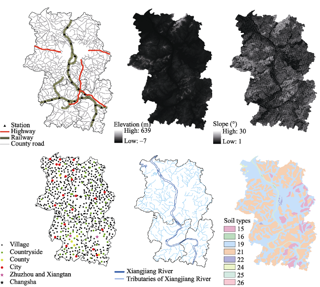
Figure 3 The spatial distribution of driving factors in the Chang-Zhu-Tan urban agglomeration

2.3 Methods

2.3.1 Prediction of demand areas
The correct selection of the area demand forecasting model is critical to guarantee the reliability of the CLUE-S model predictive results. In this study, the gray forecasting model, GM (1.1), was used to predict the demand areas of construction land in the Chang-Zhu-Tan. The constructive idea of the GM (1.1) model is to randomly generate a time series as the original sequence, accumulating the new sequence by time (Jiang et al., 2015; Yuan et al., 2016). According to GM (1.1) model, the demand area of construction land of 2014-2023 was forecasted by using the data of 1995-2009, and the time response function:
x(t+1)=5076.07e0.06t-4670.98
where x is the predicted area of construction land. t is the time, or the year.
2.3.2 Simulation of spatial distribution
The Autologistic model is based on the general logic regression equation, and the autocorrelation variable is introduced as the internal driving factor to eliminate the influence of the spatial autocorrelation effect. At present, the model has been widely used in ecological diversity modeling (Wu et al., 2009; Augustin et al., 1996). In this research, Autologistic regression result of construction land was:
$\log \left( \frac{{{P}_{0}}}{1-{{P}_{0}}} \right)=-0.38{{x}_{1}}-0.04{{x}_{2}}+0.11{{x}_{3}}+0.07{{x}_{4}}-0.08{{x}_{5}}+8.82auto\operatorname{cov}+0.40$
where P0 indicates the possibility that a particular type of ecosystem may appear in a space unit. xn represents driving factors with higher significance, x1 represents elevation, x2 represents distance from highways, x3 represents slope, x4 represents aspect and x5 represents soil types. autocov means variables of spatial autocorrelation.
The CLUE-S has very powerful spatial computing ability, and it is based on the system theory to simulate land use change. The model is an effective tool for dynamically simulating the spatial and temporal changes of the complex land use system in the region. The CLUE-S model is based on the principle of empirical statistics, and consists of two components, the spatial analysis module and the non-spatial land demand module. In the spatial analysis module, according to the land-use type probabilities and land-use rules, it is transformed into suitable land-use type, and simulated the land-use (Verburg et al., 2002; Jiang et al., 2015). The non-spatial analysis module calculates the area change of land-use types over a period based on natural, social and economic analysis, or based on the accumulated data of the various types of land in the past time series. Add the results of GM (1.1) and Autologistic model into the CLUE-S model generates the spatial distribution of the target year.
2.3.3 Landscape indexes of construction land area
Four landscape indexes calculated by Flagstats software were used to describe the spatial distribution of construction land expansion.
Contiguity index assesses the spatial connectedness or contiguity. Aggregation index is calculated from an adjacency matrix, which shows the frequency with which different pairs of patch types (including like adjacencies between the same patch type) appear side-by-side on the map. The patch cohesion index measures the physical connectedness of the corresponding patch type. In addition, Euclidean nearest-neighbor distance is perhaps the simplest measure of patch context and has been used extensively to quantify patch isolation.
$CONTIG=\frac{\left[ \frac{\sum\limits_{r=1}^{z}{{{C}_{ijr}}}}{{{a}_{ij}}^{\text{*}}} \right]-1}{v-1}\begin{matrix} {} & {} & AI=\left[ \frac{{{g}_{ii}}}{\max \to {{g}_{ii}}} \right] \\\end{matrix}\cdot (100)$
$Cohesion=\left[ 1-\frac{\sum\limits_{j=1}^{n}{{{P}_{ij}}^{*}}}{\sum\limits_{j=1}^{n}{{{P}_{ij}}^{*}\sqrt{{{a}_{ij}}^{*}}}} \right]\cdot {{\left[ 1-\frac{1}{\sqrt{Z}} \right]}^{-1}}\cdot \left( 100 \right)\begin{matrix} {} & {} & ENN={{h}_{ij}} \\\end{matrix}$
where Cijr represents contiguity value for pixel r in patch ij. v presents sum of the values in a 3-by-3 cell template. $a{{_{j}^{*}}_{i}}$ represents area of patch ij in terms of number of cells. gii represents number of like adjacencies between pixels of patch type i based on the single-count method. max→gii represents maximum number of like adjacencies between pixels of patch type i based on the single-count method.$p{{_{j}^{*}}_{i}}$represents perimeter of patch ij in terms of number of cell surfaces. $a{{_{j}^{*}}_{i}}$represents area of patch ij in terms of number of cells. Z represents total number of cells in the landscape. hij represents distance from patch ij to the nearest neighboring patch of the same type, based on patch edge-to-edge distance, computed from cell center to cell center.
2.3.4 Gravity center of construction land area
The concept of gravity center originated from physics. In this study, the theory of gravity center was used to analyze the spatial development and gravity center of construction land, and also determined how they changed over time. Due to the differences between regions in the level and speed of development, the gravity center is often in a state of change which reflects the changing track of regional development differences.
Mi is the “weight” in the sense of a certain attribution in a region, so the regional center of gravity coordinates in the sense of attribution is:
${{x}_{m}}=\frac{\sum\limits_{i=1}^{n}{{{M}_{i}}{{X}_{i}}}}{\sum\limits_{i=1}^{n}{{{M}_{i}}}}\begin{matrix} {} & {{y}_{m}} \\\end{matrix}=\frac{\sum\limits_{i=1}^{n}{{{M}_{i}}{{Y}_{i}}}}{\sum\limits_{i=1}^{n}{{{M}_{i}}}}$
where Xi and Yi represent the longitude and latitude coordinates of the center; xm and ym represent the longitude and latitude coordinates of the gravity center.
2.3.5 Verification of simulation results accuracy
Because there are errors in the simulation process, many scholars pay great attention to the accuracy test of model simulation results. In this research, the Kappa coefficient and overlap rate were calculated by comparing the pixel of two layers (actual classified data and simulated result) one by one, so as to reflect the simulation accuracy. The overlap rate was to subtract the pixel of two layers by using the raster calculator in ArcGIS, and the pixel whose attribute was zero was the correct pixel of the simulation result. The formula of Kappa coefficient (Pontius, 2000) is:
$Kappa=\frac{{{P}_{o}}-{{P}_{c}}}{{{P}_{p}}-{{P}_{c}}}$
where Po represents the percentage of the simulated correct raster in the total raster. Pc represents the expected simulation proportion in random situation. Pp represents the current ideal simulation proportion.

3 Result

3.1 Spatial-temporal expansion of construction land

Autologistic-CLUE-S model was used to simulate the construction land area of the Chang- Zhu- Tan in 2009 and 2014, and the validation was carried out using remote sensing data through Kappa coefficient and overlap rate. The Kappa coefficients were both above 0.70, and the overlap rates were both over 92.33%, indicating that the model had good results in simulating the construction land in 2009 and 2014, that is, the model was effective in simulating urban expansion. Therefore, the construction land of the Chang-Zhu-Tan in 2019-2023 could be simulated by this model (Figure 4).
Figure 4 Simulation results of Autologistic-CLUE-S model for the Chang-Zhu-Tan urban agglomeration from 2009 to 2023
Through visual interpretation, from 1995 to 2014, the Chang-Zhu-Tan construction area grew very rapidly. However, each city had its own development rules and directions, having presented obvious different characteristics at different stages. From 1995 to 2000, the Chang-Zhu-Tan construction land expansion was relatively slow, having shown a steady trend in growth. By 2005, the urban agglomerations in the five years had developed rapidly compared with the previous years. Zhuzhou and Xiangtan began to develop, but the main city of growth was still Changsha. After 2005, the growth of construction land in Changsha slowed down and Zhuzhou’s and Xiangtan’s accelerated.
The area and growth rate of the Chang-Zhu-Tan and various cities during 1995-2014 were calculated by a statistical tool. Overall, the Chang-Zhu-Tan construction area increased from 372.28 km2 to 864.37 km2 from 1995 to 2014 (Figure 5). The increment was 492.09 km2, or 25.90 km2 per year. Among them, Changsha, Zhuzhou and Xiangtan, respectively, increased to 330.30 km2, 91.96 km2 and 69.83 km2. The expansion speed of the three cities gradually accelerated since 2000. Between 2005 and 2009, Changsha entered a period of rapid development with the growth rate of 29.65%. From 2009, the development pace of Zhuzhou and Xiangtan had speeded up, with the growth rates of 31.61% and 26.71% respectively. According to the simulation result, the construction land area of the Chang-Zhu-Tan may reach 1125.38 km2 and 1327.23 km2 in 2019 and 2023, with the growth rate of 30.20% and 17.94%. It was speculated that the Chang-Zhu-Tan would continue to maintain a rapid development from 2014 to 2019. But the development speed will slow down after 2019.
Figure 5 Construction land area expansion of Chang-Zhu-Tan urban agglomeration and each city from 1995 to 2023

3.2 Spatial move of gravity center

This research not only studied the spatial expansion of construction land in the Chang- Zhu- Tan, but also focused on the evolution path of construction land’s gravity center (Figure 6). From 1995 to 2014, the gravity center of the construction land in Changsha moved to the north, and it was found going to shift to the southeast through calculating the simulation results of the gravity center of 2019 and 2023. In Zhuzhou, from 1995 to 2014, the gravity center at first moved to the southwest, and later moved to the northwest. Hence, Zhuzhou gradually docked with Changsha and Xiangtan. As can be seen from the figure, the development of the northeastern part in Zhuzhou will become much more rapid in the future. About Xiangtan, the movement of the gravity center of the past few years had no similar laws and direction, and the moving distance was very short. However, from the end of 2007, with “a resource-saving and environment-friendly society” of the Chang-Zhu-Tan being determined to establish and promoted, the gravity center of construction land kept moving to the northeast.
Figure 6 Changing of gravity center in the Chang-Zhu-Tan urban agglomeration from 1995 to 2023
Taking Chang-Zhu-Tan as a whole, the gravity center of urban agglomeration moved to the south, except its moving to the north for some distance in 2009. And in the future, it will continue moving to the southeast.

3.3 The direction of construction land expansion

To describe the expansion of the Chang-Zhu-Tan specifically, there is a requirement of using district as a unit and putting the above results into the analysis (Figure 7). From 1995 to 2014, the more rapid expansion areas of Changsha were Wangcheng district, Yuelu district, Kaifu district and Yuhua district. And according to the expansion result of gravity center, those two results remained consistent. Since the beginning of the Tenth Five-Year Plan (2011-2015), Changsha started to be divided into groups in order to promote the rapid development of the city. After 2014, the development focus of Changsha might move southward, and the main districts might be Yuelu district, Yuhua district, and Changsha county. From 1995 to 2014, Tianyuan district was the more rapid expansion area in Zhuzhou. As a consequence, this led to the continuous reduction of the distance between Zhuzhou and Xiangtan. Furthermore, the future development focus of Zhuzhou will likely move to the northeast. Yuhu district and Yuetang district were the key construction areas in the overall planning of Xiangtan. Therefore, these two regions were also the areas with relatively rapid development. The direction of urban development was mainly concentrated in the northeast, in order to gradually dock with Changsha and Zhuzhou.
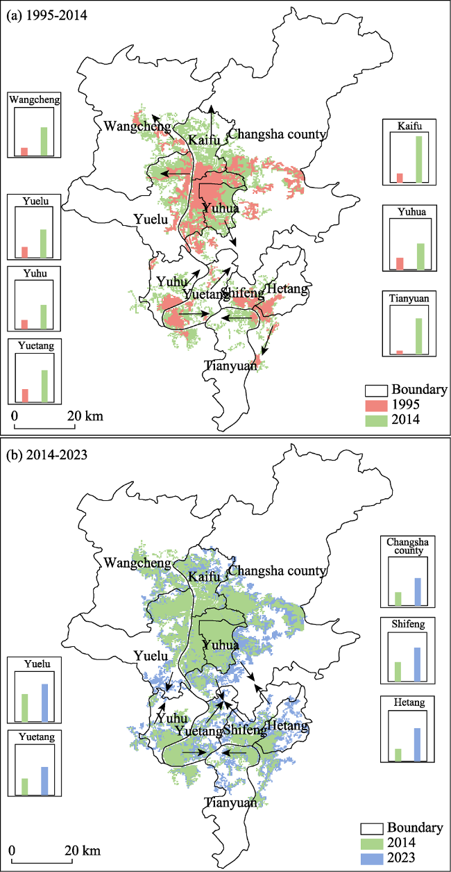
Figure 7 The development direction of construction land expansion in the Chang-Zhu-Tan urban agglomeration (the histogram represented the area of each district)
Since 2008, the three cities, Changsha, Zhuzhou, and Xiangtan, began to change gradually from their own development into a common and gathering development. Also, the distance between the boundaries of the three cities was getting closer.

3.4 Aggregation of the urban boundary buffers

The buffers of 1 km, 2 km and 3 km were used to observe the gathering of urban boundaries. At the same time, the shortest distance between the cities was calculated by averaging the shortest distances between each two cities in the boundary area.
It can be seen that the area of construction land in the buffers was increased (Figure 8), which was in line with the trend of the urban agglomeration development defined in the government plan. Especially after 2009, the area grew very rapidly. And according to the simulation results, the area within the buffers in 2019 and 2023 will show a multiplied growth trend. Besides, the distances between the three cities had been decreasing. Among them, the distance between Changsha and Xiangtan, Xiangtan and Zhuzhou reduced to 0. Furthermore, the two periods of rapid decline were 2000 to 2005 and 2009 to 2014.
Figure 8 The Change of distance and area in the urban boundary buffers from 1995 to 2023

3.5 Analysis of dispersion or aggregation in Chang-Zhu-Tan

In this part, four landscape indexes and the above results were used to synthetically describe the spatial distribution of construction land expansion (Figure 5). The Contig_AM, AI indexes and Cohesion index are related to the degree of aggregation. From 1995 to 2023, although there was a slight decrease in 2014 and 2023, three indexes of the Chang-Zhu-Tan showed an overall upward trend. The Contig_AM and AI indexes of Zhuzhou and Xiangtan declined continuously from 2000 to 2014, and the reason for the decline might be the dispersal expansion of the urban non-core area. The Cohesion index of Changsha had kept the trend of rising except for 2000 which might be due to the insignificant expansion of construction land and the disappearance of many small patches in Changsha in 2000, resulting in longer distances between the patches. This index of Zhuzhou declined from 2005 to 2009, and Xiangtan’s fell in 2009. This phenomenon might be due to the expansion of the city in the suburbs.
Enn_MN is the index that calculates the closest distance between patches. All the results had a very similar trend that firstly rose and then fell, indicating that since 2005, urban agglomerations and cities were both constantly gathering and expanding. This was very consistent with the integration of the Chang-Zhu-Tan.
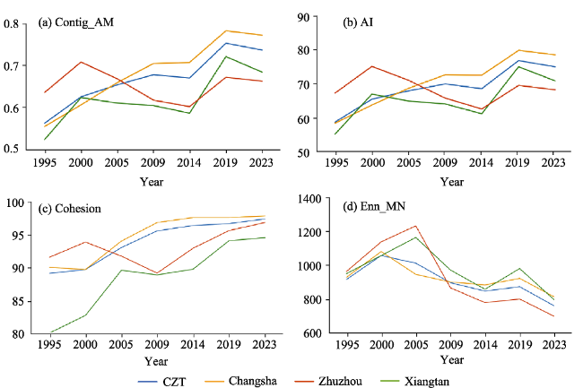
Figure 9 The change regulation of four landscape indexes, including Contiguity index (Contig_AM), Aggregation index (AI), Cohesion index (Cohesion), and Euclidean nearest-neighbor distance (Enn_MN)

4 Discussion

4.1 The significance of this research

This research studied the changes of construction land in the Chang-Zhu-Tan from 1995 to 2023 by analyzing the area of the Chang-Zhu-Tan, the gravity center of the construction land, the minimum distance in the urban boundary buffers and the landscape indexes. The results indicated that: from 1995 to 2014, urban agglomeration had shifted from their separate development to the gathering development, and the distances between cities got smaller or even reduced to 0. After 2014, the urban area in the buffers between the three cities developed more quickly, and gradually formed the integration of urban agglomeration. Overall, this paper not only used remote sensing images to monitor the past development of urban agglomeration, but also used model to predict the future development. And according to the research results of Liu and Chen (2017) and Zou et al. (2017), the urbanization process of Chang-Zhu-Tan urban agglomeration was very rapid, but the speed has decreased in recent years, and the development direction of Chang-Zhu-Tan was northwest to southeast. These results were very consistent with our results. In this way, the result of this research might provide some reference for the government to formulate the future plans.
Then, previous studies usually focused on spatial-temporal change in the urban expansion, while this study added the movement of the gravity center, which highlighted the direction of construction land expansion. Gravity center was mostly used in economy and energy in past studies, so this method was used in the study of construction land to provide more references for the future urban development research. In addition, this paper not only analyzed a single city, but also discussed the relationship and development between cities and the whole urban agglomeration. It also offered some references for the study of urban agglomeration.

4.2 Coincidence between research results and policies

Since 1990, the government planning and policies of Changsha, Zhuzhou and Xiangtan were collected and combined with the above results to analyze the coincidence degree. Around 1995, the main goal of the three cities was to basically form a perfect urban system, so that all the districts and counties could form a whole. Therefore, from the beginning of 1995, the city mainly focused on the development and expansion. And in that period, the integration policy of the Chang-Zhu-Tan had not yet formed, so the planning had not highlighted the coordinated development with other two cities. Around 2014, the development of the three cities entered a stable period, the main objective of which was to moderately expand the scale of urban areas, improve the infrastructure construction and functions and the quality of cities. According to the planning, around 2023, Changsha will develop to the east and the south, Zhuzhou will grow to the west and the northeast, and Xiangtan will expand to the east and the north, which is very consistent with the above result of gravity center. The result of the model simulation was well coincided with the planning as well. However, in December 2007, the National Development and Reform Commission approved the Changsha-Zhuzhou-Xiangtan urban agglomeration as a “National Resource-saving and Environment-friendly Society Integrated Support Reform Experimental Zone”. Since 2008, Changsha, Zhuzhou and Xiangtan have been gradually connected, and have responded positively to the relevant policies of integration. Then the gravity center of the Chang-Zhu-Tan has been shifting to the south, for the reason that the planning identified to develop mainly in the south.

4.3 Uncertainty and future research direction

However, this simulation model could be uncertain. First, it needs to solve the quantitative problems of some human driving forces, for example, policy factors. Second, the resolution of the remote sensing data used in this research was 30 m, which might lead to the deviation of the research results. Third, the time chosen as the time nodes in this study were 1995, 2000, 2005, 2009 and 2014, which was a long time span and should be shortened in the future research. At the same time, future studies will focus on the urban boundary buffers.

5 Conclusions

In this research, the study area is the core area of the Chang-Zhu-Tan urban agglomeration, and there are two types of data were cited, including Landsat remote sensing images and Autologistic-CLUE-S model simulation data. The expansion of its construction land was studied based on the method of gravity center, the change of development direction, the distance in the urban boundary buffers and the landscape index. The findings are mainly as follows: (1) From 1995 to 2014, the construction land of Changsha, Zhuzhou and Xiangtan expanded rapidly. And with the continuous integration of the Chang-Zhu-Tan, the distances between the three cities have continued to be shortened, and the development gradually got coordinated. (2) At first, the development direction of cities’ gravity centers was dispersed, and later concentrated gradually. And the gravity center of the Chang-Zhu-Tan moved to the south. (3) With reviewing the planning and policies in the study area, it was found that the results of this research were in good agreement with them. In general, this research made clear the current status of the construction land expansion of the Chang-Zhu-Tan, and the possible trend of development, and provided some auxiliary basis for the future planning.
[1]
Augustin N H, Mugglestone M A, Buckland S T , 1996. An autologistic model for the spatial distribution of wildlife. Journal of Applied Ecology, 33(2):339-347.

[2]
Castella J C, Kam S P, Quang D D et al., 2007. Combining top-down and bottom-up modelling approaches of land use/cover change to support public policies: Application to sustainable management of natural resources in northern Vietnam. Land Use Policy, 24(3):531-545.

[3]
Chen Y, Chen Z G, Xu G L et al., 2016. Built-up land efficiency in urban China: Insights from the general land use plan (2006-2020). Habitat International, 51:31-38.

[4]
Chen Z G, Wang Q, Huang X J et al., 2007. Movement of urban agglomeration gravity and its driving forces in the Changjiang (Yangtze) Delta of China. Scientia Geographica Sinica, 27(4):457-462. (in Chinese)

[5]
Deng F F, Huang Y Q , 2004. Uneven land reform and urban sprawl in China: The case of Beijing. Progress in Planning, 61(3):211-236.

[6]
Fu J, Gao Z G, Huang L Y et al., 2011. The movement route of consumption gravity center of Xinjiang from 1965 to 2009 based on GIS. Procedia Earth and Planetary Science, 2(1):321-326.

[7]
Geist H J, Lambin E F , 2002. Proximate causes and underlying driving forces of tropical deforestation. Bioscience, 52(2):143-150.

[8]
Han L J, Zhou W Q, Li W F , 2016. Fine particulate (PM2.5) dynamics during rapid urbanization in Beijing, 1973-2013. Scientific Reports, 6:23604.

[9]
Hu L, Jiang C Y, Li Z B et al., 2011. Evolution path analysis of economic gravity center and air pollutants gravity center in Shaanxi province. Advanced Materials Research, 361- 363:1359-1363.

[10]
Jiang W G, Chen Z, Lei X et al., 2015. Simulating urban land use change by incorporating an autologistic regression model into a CLUE-S model. Journal of Geographical Sciences, 25(7):836-850.

[11]
Jiang W G, Chen Z, Lei X et al., 2016. Simulation of urban agglomeration ecosystem spatial distributions under different scenarios: A case study of the Changsha-Zhuzhou-Xiangtan urban agglomeration. Ecological Engineering, 88:112-121.

[12]
Jiang W G, Deng Y, Tang Z H et al., 2017. Modelling the potential impacts of urban ecosystem changes on carbon storage under different scenarios by linking the CLUE-S and the InVEST models. Ecological Modelling, 345:30-40.

[13]
Li Y F, Liu G H, Huang C , 2017. Dynamic changes analysis and hotspots detection of land use in the central core functional area of Jing-Jin-Ji from 2000 to 2015 based on remote sensing data. Mathematical Problems in Engineering, 2017(3):1-16.

[14]
Liu D D, Chen N C , 2017. Satellite monitoring of urban land change in the middle Yangtze River Basin urban agglomeration, China between 2000 and 2016. Remote Sensing, 9(11):1086.

[15]
Lourdes L, Karina Z, Pedro L et al., 2011. A dynamic simulation model of land cover in the Dulce Creek Basin, Argentina. Procedia Environmental Sciences, 7:194-199.

[16]
Lv Z Q, Dai F Q, Sun C , 2012. Evaluation of urban sprawl and urban landscape pattern in a rapidly developing region. Environmental Monitoring and Assessment, 184(10):6437-6448.

[17]
Pal M, Foody G M , 2010. Feature selection for classification of hyperspectral data by SVM. IEEE Transactions on Geoscience and Remote Sensing, 48(5):2297-2307.

[18]
Peng J, Zhao M Y, Guo X N et al., 2017. Spatial-temporal dynamics and associated driving forces of urban ecological land: A case study in Shenzhen City, China. Habitat International, 60:81-90.

[19]
Price B, Kienast F, Seidl I et al., 2015. Future landscapes of Switzerland: Risk areas for urbanisation and land abandonment. Applied Geography, 57:32-41.

[20]
Pontius R G , 2000. Quantification error versus location error in comparison of categorical maps. Photogrammetric Engineering and Remote Sensing, 66(8):1011-1016.

[21]
Puertas O L, Henríquez C, Meza F J , 2014. Assessing spatial dynamics of urban growth using an integrated land use model. Application in Santiago Metropolitan Area, 2010-2045. Land Use Policy, 38:415-425.

[22]
Quan B, Xiao Z K, Römkens M J M et al., 2013. Spatiotemporal urban land use changes in the Changzhutan region of Hunan province in China. Journal of Geographic Information System, 5(2):136-147.

[23]
Rafiee R, Mahiny A S, Khorasani N et al., 2009. Simulating urban growth in Mashad City, Iran through the SLEUTH model (UGM). Cities, 26(1):19-26.

[24]
Seto K C, Fragkias M , 2005. Quantifying spatiotemporal patterns of urban land-use change in four cities of China with time series landscape metrics. Landscape Ecology, 20(7):871-888.

[25]
Silva E A, Clarke K C , 2002. Calibration of the SLEUTH urban growth model for Lisbon and Porto, Portugal. Computers, Environment and Urban Systems, 26(6):525-552.

[26]
Sun Y, Zhao S Q , 2018. Spatiotemporal dynamics of urban expansion in 13 cities across the Jing-Jin-Ji urban agglomeration from 1978 to 2015. Ecological Indicators, 87:302-313.

[27]
Tang F H, Chen L L , 2011. The evolution of regional differences of Chang-Zhu-Tan urban agglomeration since the 1990. Geographical Research, 30(1):94-102. (in Chinese)

[28]
Vasenev V I, Stoorvogel J J, Leemans R et al., 2018. Projection of urban expansion and related changes in soil carbon stocks in the Moscow Region. Journal of Cleaner Production, 170:902-914.

[29]
Veldkamp A, Fresco L O , 1996. CLUE: A conceptual model to study the conversion of land use and its effects. Ecological Modelling, 85(2/3):253-270.

[30]
Veldkamp A, Fresco L O , 1997. Exploring land use scenarios, an alternative approach based on actual land use. Agricultural Systems, 55(1):1-17.

[31]
Verburg P H, Schulp C J E, Witte N et al., 2006. Downscaling of land use change scenarios to assess the dynamics of European landscapes. Agriculture, Ecosystems and Environment, 114(1):39-56.

[32]
Verburg P H, Soepboer W, Veldkamp A et al., 2002. Modeling the spatial dynamics of regional land use: The CLUE-S model. Environmental Management, 30(3):391-405.

[33]
Wang C D, Wang Y T, Wang R Q et al., 2018. Modeling and evaluating land-use/land-cover change for urban planning and sustainability: A case study of Dongying city, China. Journal of Cleaner Production, 172:1529-1534.

[34]
Wang W W, Zhang M, Li P , 2014. Exploring temporal and spatial evolution of global energy production and consumption. Renewable and Sustainable Energy Reviews, 30:943-949.

[35]
Wei Y D, Li H, Yue W Z , 2017. Urban land expansion and regional inequality in transitional China. Landscape and Urban Planning, 163:17-31.

[36]
Wu D Q, Liu J, Zhang G S et al., 2009. Incorporating spatial autocorrelation into cellular automata model: An application to the dynamics of Chinese tamarisk (Tamarix Chinensis Lour.). Ecological Modelling, 220(24):3490-3498.

[37]
Wu Y Z, Zhang X L, Shen L Y , 2011. The impact of urbanization policy on land use change: A scenario analysis. Cities, 28(2):147-159.

[38]
Xu J H, Zhao Y, Zhong K W et al., 2018. Measuring spatio-temporal dynamics of impervious surface in Guangzhou, China, from 1988 to 2015, using time-series Landsat imagery. Science of the Total Environment, 627:264-281.

[39]
Yang Y Y, Liu Y S, Li Y R et al., 2018. Quantifying spatio-temporal patterns of urban expansion in Beijing during 1985-2013 with rural-urban development transformation. Land Use Policy, 74:220-230.

[40]
Yu B L, Shu S, Liu H X et al., 2014. Object-based spatial cluster analysis of urban landscape pattern using nighttime light satellite images: A case study of China. International Journal of Geographical Information Science, 28(11):2328-2355.

[41]
Yuan C Q, Liu S F, Fang Z G , 2016. Comparison of China’s primary energy consumption forecasting by using ARIMA (the autoregressive integrated moving average) model and GM (1, 1) model. Energy, 100:384-390.

[42]
Zeng C, Liu Y L, Stein A et al., 2015. Characterization and spatial modeling of urban sprawl in the Wuhan Metropolitan Area, China. International Journal of Applied Earth Observation and Geoinformation, 34(1):10-24.

[43]
Zeng C, Yang L D, Dong J N , 2017. Management of urban land expansion in China through intensity assessment: A big data perspective. Journal of Cleaner Production, 153:637-647.

[44]
Zhang Y, Zhang J Y, Yang Z F et al., 2012. Analysis of the distribution and evolution of energy supply and demand centers of gravity in China. Energy Policy, 49(10):695-706.

[45]
Zhao X F, Huang X J, Zhang X Y et al., 2010. Evolution of economic and COD, SO2, TSP emission gravity centers in Jiangsu province. Resources and Environment in the Yangtze Basin, 19(3):225-230. (in Chinese)

[46]
Zhou W Q, Huang G L, Cadenasso M L , 2011. Does spatial configuration matter? Understanding the effects of land cover pattern on land surface temperature in urban landscapes. Landscape and Urban Planning, 102(1):54-63.

[47]
Zou Y H, Peng H Q, Liu G et al., 2017. Monitoring urban clusters expansion in the middle reaches of the Yangtze River, China, using time-series nighttime light images. Remote Sensing, 9(10):1007.

Outlines

/