Vegetation dynamics dominate the energy flux partitioning across typical ecosystem in the Heihe River Basin: Observation with numerical modeling
WANG Pei
,
LI Xiaoyan
,
TONG Yaqin
,
HUANG Yongmei
,
YANG Xiaofan
,
WU Xiuchen
Expand
State Key Laboratory of Earth Surface Processes and Resource Ecology, Faculty of Geographical Science, Beijing Normal University, Beijing 100875, China
Wang Pei (1978–), PhD and Associate Professor, specialized in ecohydrology, isotope hydrology. E-mail: peiwang@bnu.edu.cn
Received date: 2018-10-23
Accepted date: 2019-02-20
Online published: 2019-12-11
Supported by
The Strategic Priority Research Program of Chinese Academy of Sciences(No.XDA20100102)
National Natural Science Foundation of China(No.41730854)
National Natural Science Foundation of China(No.41671019)
Projects by the State Key Laboratory of Earth Surface Processes and Resource Ecology
Understanding the controls on seasonal variation of energy partitioning and separation between canopy and soil surface are important for qualifying the vegetation feedback to climate system. Using observed day-to-day variations of energy balance components including net radiation, sensible heat flux, latent heat flux ground heat flux, and meteorological variables combined with an energy-balanced two-source model, energy partitioning were investigated at six sites in Heihe River Basin from 2014 to 2016. Bowen ratio (β) among the six sites exhibited significant seasonal variations while showed smaller inter-annual fluctuations. All ecosystems exhibit a “U-shaped” pattern, characterized by smaller value of β in growing season, with a minimum value in July, and fluctuating day to day. During the growing season, average Bowen ratio was the highest for the alpine swamp meadow (0.60 ± 0.30), followed by the desert riparian forest Populus euphratica (0.47 ± 0.72), the alpine desert(0.46 ± 0.10), the Tamarix ramosissima desert riparian shrub ecosystem (0.33 ± 0.57), alpine meadow ecosystem (0.32 ± 0.17), and cropland ecosystem (0.27 ± 0.46). The agreement of Bowen ratio between simulated and observed values demonstrated that the two-source model is a promising tool for energy partitioning and separation between canopy and soil surface. The importance of biophysical control explains the convergence of seasonal and annual patterns of Bowen ratio for all ecosystems, and the changes in Bowen ratio showed divergence among varied ecosystems because of different physiological responses to energy flow pathways between canopy and soil surface.
WANG Pei, LI Xiaoyan, TONG Yaqin, HUANG Yongmei, YANG Xiaofan, WU Xiuchen. Vegetation dynamics dominate the energy flux partitioning across typical ecosystem in the Heihe River Basin: Observation with numerical modeling[J]. Journal of Geographical Sciences, 2019, 29(9): 1565-1577. DOI: 10.1007/s11442-019-1677-z
1 Introduction
Plants are a primary conduit for returning terrestrial water to the atmosphere while mediating albedo and roughness (Chapin et al., 2002), thereby exerting a strong effect on hydrologic/energy fluxes of the terrestrial-atmospheric system (Burakowski et al., 2018). Plant transpiration (T) is the largest component of the terrestrial-atmosphere water/energy flux, accounting for somewhere between 50% and 90% of annual global land-surface water flux (Good et al., 2015; Jasechko et al., 2013; Maxwell and Condon, 2016). Vegetation exerts strong feedback to climate by modifying the energy, momentum, and hydrologic balances of the land surface (Arora et al., 2002; Takle et al., 2015). Therefore, climate feedback from vegetation is mainly attributable to its physiological properties (in particular, leaf area index (LAI, the ratio of leaf to ground area), stomatal resistance, and rooting depth), albedo, surface roughness, and effect on soil moisture (Arora et al., 2002). The seasonal rhythm of ecosystem energy partition emerges from interactions among climate, plant functional traits, and ecosystem structure. However, the variability of energy partitioning between sites and years has been uncertain and inconsistent.
The Bowen ratio (β), an important index of ecosystem energy partitioning, was defined as the ratio of sensible (H) to latent heat fluxes (lET) from the earth’s surface up into the air (Bowen, 1926), which heavily influences ecosystem microclimates and hydrological cycles at both regional and global scales via its effect on the warming extent of available energy to the land surface air (Ning et al., 2019). The β values vary with different surface types, ranging from 0.1 over the oceans to 10 over the desert regions (https://en.wikipedia.org/wiki/ Bowen _ratio). Thus, β is also a good indicator of the ecosystem biophysical properties. It is necessary to partition energy fluxes into soil and canopy surface to provide useful information to develop vegetation models and reduce agricultural water use. However, few studies have considered canopy and soil surface energy partitioning separately and conducted a comprehensive assessment. Generally, β can be estimated as the psychrometric constant times the ratio of potential temperature difference to mixing ratio difference, where the differences are measured between the same two heights in the atmospheric surface layer. Based on the eddy covariance measurements, the β can be calculated directly by using the measured sensible (H) and latent heat fluxes (lET). However, those are fundamentally different methods, and both types of method lack the complex interaction between soil, vegetation and atmosphere that occurs in ecosystems. Two-source model is a promising tool for integrating the energy/water processes with separate soil and canopy layer in terrestrial ecosystems and has the advantage of enabling assessment of energy partitioning between canopy and soil surface. The well-known two-source model (e.g. Shuttleworth-Wallace model) enables us to partition latent heat flux into soil evaporation and transpiration, but the model does not exactly consider the radiation/energy balances at vegetation and ground surfaces. The two-source model (Wang and Yamanaka, 2014), considering the radiation/energy balances at vegetation and ground surfaces, achieved good performance in partitioning energy flux in the humid grasslands of Japan (Wang and Yamanaka, 2014; Wang et al., 2015), the cropland ecosystem (Wang et al., 2016c), and arid and semiarid grassland in Inner Mongolia of China (Wang et al., 2018).
Heihe River Basin (HRB), the second largest inland river basin in the arid region of northwestern China, is one of the most instrumented and well-studied river basins in China (Cheng, 2009; Li et al., 2013). Continuous records of surface energy balance are currently available for the typical ecosystems (Liu et al., 2013). However, the seasonal and inter-annual variations of energy petitioning in response to vegetation dynamics across various ecosystems within the HRB have yet to be analyzed. Few studies assess the energy partitioning between soil and canopy surface separately. The objectives of the present study were to: (1) investigate the seasonality and its controls of energy partitioning in the typical ecosystem in the HRB; (2) clarify plant effects on the energy partitioning in the typical ecosystem in the HRB.
2 Materials and methods
2.1 Study site
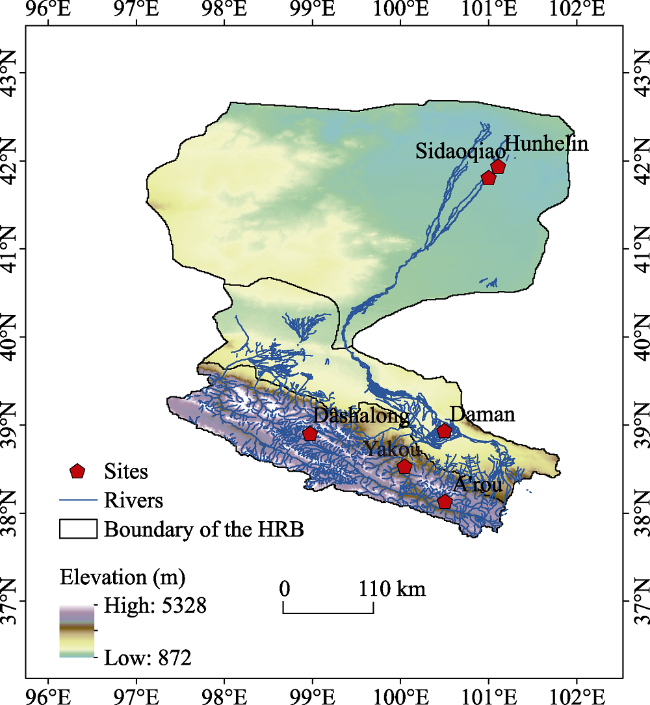
Under the framework of the HiWATER (http://hiwater.westgis.ac.cn/), hydrometeorological observation network dataset, including eddy coevolution (EC) systems and automatic weather stations (AWS), were deployed at typical ecosystem across upstream, middle stream, and downstream in the Heihe River Basin (97.1 E-102.0°E and 37.7°N-42.7°N) for ecohydrological and micrometeorological monitoring. The total area of the HRB is 14.3 million km2 which integrates alpine glaciers, alpine grassland, oases, and the Gobi desert (Cheng et al., 2014). In the upper reaches in the Qilian Mountains, at an altitude between 1674 and 5564 m, the climate is cold and arid. With characteristics of wet and cold climate (an average annual temperature of 0.54℃) and an average annual precipitation of 300-600 mm, the vegetation distribution is more obvious in the vertical zone, which mainly consists of sparse alpine vegetation, alpine meadows, swamp meadow and alpine desert. The middle reaches, at an altitude between 1352 m and 1700 m, have a temperate continental arid climate with an annual average precipitation of 90-160 mm and an annual evaporation of 2000-2500 mm. The vegetation type is natural and artificial oases, which are the areas with the greatest intensity of human activity. The lower reaches have an altitude less than 1352 m and are more arid, with rare precipitation and strong evapotranspiration. The average annual temperature is 8.7℃, the average annual rainfall is 36.6 mm, and the vegetation is mainly desert and riparian forest. There are series of hydrometeorological observatory in the upstream, midstream and downstream of the HRB (Liu et al., 2018), covering the main vegetation types of the HRB. As shown in Figure 1, the alpine meadow and alpine swamp meadow, and alpine desert ecosystems in the upper reaches, the cropland ecosystem in the middle reaches, and the Tamarix ramosissima Ledeb, Populus euphratica ecosystems in the lower reaches were selected for investigation in the present study. All sites have continuous observation data from eddy covariance systems (EC) and automatic weather stations (AWS) from January 2014 to December 2016. Table 1 lists detailed descriptions of each ecosystem.
Figure 1 Geographic location of the study sites within the Heihe River Basin
Table 1 Description of the study sites in the Heihe River Basin
River section
Site
Longitude
Latitude
Altitude (m)
Dominant vegetation type
EC height (m)
Energy close
Upstream
Yakou
100.23°E
38.02°N
4101
Alpine meadow
3.5
0.53-0.55
Dashalong
98.94°E
38.84°N
3739
Alpine swamp meadow
4.5
0.74-0.87
A’rou
100.46°E
38.05°N
3044
Alpine meadow
3.5
0.95-0.96
Midstream
Daman
100.37°E
38.86°N
1556
Cropland
4.5
0.75-0.89
Downstream
Hunhelin
101.13°E
41.99°N
874
P.euphratica
22
0.87-0.91
Sidaoqiao
101.14°E
42.00°N
873
T.ramosissima
8
0.85-0.89
Note: EC means eddy covariance; EC height means EC systems were mounted on towers above the canopy heights.
2.2 Plant dynamics and continuous micrometeorological and eddy covariance measurements
The GLASS leaf area index (LAI) products (http://glassproduct.bnu.edu.cn/) from Beijing Normal University, available every 8 days and interpolated onto a daily time interval, were used to represent vegetation dynamics in this study. Vegetation heights of riparian forest in the lower reaches were acquired by a field quadrat survey, and vegetation heights of alpine meadow in the upper reaches were obtained by reference to a research dataset of ecohydrological transects in the HRB in 2013. The heights of maize in cropland were as given by Wen et al. (2016).
The study data were obtained from a hydrometeorological observation network dataset provided by HiWATER (http://hiwater.westgis.ac.cn/), which includes EC systems and AWS. The data collection has been described in detail (Liu et al., 2018; Xu et al., 2013). The EC systems were mounted on towers ranging from 3.5 to 22 m above the various canopy heights (Table 1). Post-processing calculations were performed using EdiRe (Liu et al., 2011), and the results were gap-filled using a set of general algorithms (Reichstein et al., 2005). After gap-filling, daily energy budget closure was used to elevate the EC data, which was determined by the linear regression statistics between (lET+H) and (Rn-G) (Liu et al., 2011). The energy balance closure for daily-mean dataset ranged from 53% to 96% (Figure 2), which indicated that energy balance closure problem in our sites was not a big issue. Meteorological data including air temperature (Ta, ℃), humidity (RH, %), wind speed (u, m/s), air pressure (P, Pa), soil temperature (Ts, ℃), moisture profile (θ, %), and solar radiation/soil heat flux (Rn, W m-2), were used for model input. The energy balance closure for the daily-mean datasets ranged from 74% to 96% (Table 1), which indicated that energy balance closure issue was not a big concern in our sites (Pan et al., 2017).
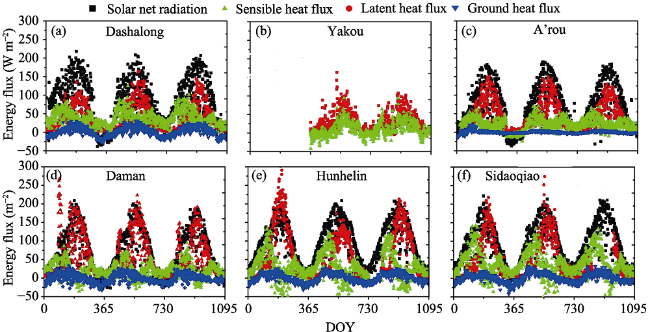
Figure 2 Seasonal day-to-day variations of observed energy flux of net radiation (Rn), sensible heat flux (H), latent heat flux (IET) and ground heat flux (G) in the Heihe River Basin from 2014 to 2016
2.3 Model description for energy partitioning into soil and plant layer
A two-layer source model was used to partition energy between plant and soil layer. The main equations of the model are illustrated in supplementary materials (Text S1). This model was chosen for the following reasons. First, this model, using the energy balance between the soil surface and the vegetation canopy and taking into account the energy interaction between them, achieved good performance in partitioning energy flux in the humid grasslands of Japan (Wang and Yamanaka, 2014; Wang et al., 2015), the cropland ecosystem of the HRB (Wang et al., 2016), and arid and semiarid grassland in Inner Mongolia of China (Wang et al., 2017; Wang et al., 2018). Second, the model uses the Newton-Raphson iteration scheme to solve the governing equations for the canopy and the ground surface separately without the need for radiometric temperature. Third, the model considers stomatal control of transpiration, including its dependence on soil moisture, and solar radiation is explicitly included. The model was localized to fit the characteristics of each ecosystem; Text S1 summarizes the parameters used for each site in this study. More details about the model can be found in Wang and Yamanaka (2014). The root mean square error (RMSE) and I index (Willmott et al., 1985; Wang and Yamanaka, 2014), as well as R2 (R is the correlation coefficient), were used to validate and test the model for energy partitioning.
2.4 Determination of Bowen ratio and partitioning between canopy and soil surface
According to the eddy covariance measurements, the β was estimated based on the measured sensible (H) divided by latent heat fluxes (lET):
β = H / lET
where H and lET are sensible (H) and latent heat flux (lET) respectively.
Based on the two-source model output, the βV was estimated based on the simulated sensible (HV) divided by transpiration fluxes (lT):
βV = HV/lT
The βG was estimated based on the simulated sensible (HG) divided by evaporation fluxes (lE):
βG = HG/lE
3 Results
3.1 Seasonal variations of energy flux for typical ecosystem
The observed day-to-day variations in energy balance components of net radiation, sensible heat flux, and latent heat flux and ground heat flux were shown at six sites in the HRB (Figure 2). Energy partitioning was dominated by latent heat, followed by sensible heat and the soil heat flux for six ecosystems during 2014-2016. Among the six ecosystems, the maximum latent heat was observed in riparian forest ecosystem of Hunhelin, followed by agriculture ecosystem of Daman and Sidaoqiao. There are larger fluctuations of lET for ecosystems of riparian forest and agriculture ecosystem than ecosystems in upstream. The detailed statistics of monthly mean dataset of latent (lET) and sensible heat flux (H) were summarized in Table 2. Using gap-filling dataset, daily energy budget closure was evaluated by the linear regression statistics between (lET+H) and (Rn-G) (Liu et al., 2011b).
Table 2 Statistics of monthly mean dataset of latent (lET) and sensible heat flux (H) of the study sites in the Heihe River Basin during 2014-2016
Site
Item
N
Mean
S.D.
Minimum
Median
Maximum
Yakou
lET
24
31.01
19.67
6.04
28.02
68.97
H
24
11.27
14.01
-7.55
13.53
37.43
A’rou
lET
36
41.13
32.84
2.74
30.36
103.23
H
36
21.10
11.80
-7.51
20.71
42.08
Dashalong
lET
36
38.79
30.02
2.31
30.62
96.19
H
36
36.85
13.35
10.48
34.96
62.68
Daman
lET
36
58.49
45.86
4.59
51.95
152.86
H
36
20.91
15.82
-5.82
17.65
52.99
Hunheklin
lET
36
61.02
61.32
1.74
29.40
223.25
H
36
30.82
29.39
-8.71
21.49
87.85
Sidaoqiao
lET
33
45.44
49.23
2.39
21.63
152.46
H
36
39.22
26.77
-4.48
38.52
100.79
3.2 Seasonal variations of Bowen ratio and vegetation dynamics for typical ecosystem
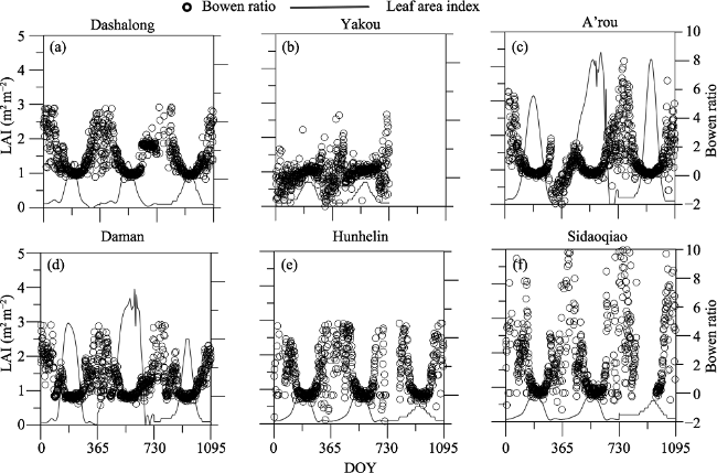
Seasonal day-to-day variations of leaf area index (LAI) and observed β for Dashalong, Ya kou, A’rou, Daman, Hunhelin and Sidaoqiao from 2014 to 2016 were shown in Figure 3.
Figure 3 Seasonal day to day variations of leaf area index (LAI) and Bowen ratio in the Heihe River Basin from 2014 to 2016
Bowen ratio (β) among the six sites exhibited significant seasonal variations with smaller inter-annual fluctuations. All ecosystems exhibit a “U-shaped” pattern, characterized by smaller value of β in growing season, with a minimum value in July, and fluctuating day to day. Statistics of measured Bowen ratio show that there is significant difference (P < 0.01) between growing season and non-growing season for all ecosystems (Table 3). We find there is negative fluctuation between leaf area index and β. There is smaller β with higher LAI during the growing season while higher β with lower LAI during non-growing season. For non-growing season, there were higher β values than growing season, indicating that there were other environmental factors (e.g. snow, freeze soil surface) rather than vegetation dominating the energy partitioning. During the growing season, average Bowen ratio was the highest for the alpine swamp meadow (0.60 ± 0.30), followed by the desert riparian forest Populus euphratica (0.47 ± 0.72), the alpine desert (0.46 ± 0.10), the Tamarix ramosissima desert riparian shrub ecosystem (0.33 ± 0.57), alpine meadow ecosystem (0.32 ± 0.17), and cropland ecosystem (0.27 ± 0.46).
Table 3 Statistics of measured Bowen ratio with daily mean dataset of the study sites for growing season and all year in the Heihe River Basin
Site
Grow season
All year
A’rou
0.32 ± 0.17
0.96 ± 0.43
Dashalong
0.60± 0.30
2.17 ± 1.44
Yakou
0.46 ± 0.10
0.21 ± 0.18
Daman
0.27 ± 0.46
1.08 ± 0.50
Hunhelin
0.33 ± 0.57
2.56 ± 1.03
Sidaoqiao
0.47 ± 0.72
3.30 ± 0.12
3.3 Bowen ratio partitioning between soil and vegetation surface
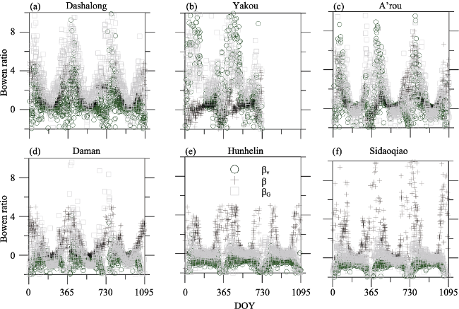
There is reasonable agreement between observed and simulated Bowen ratio (β), with high Iindex (0.64-0.85), and R2 (0.28-0.31) and lower RMSE (0.22-0.50) values of the six ecosystems (Table 4), which indicate that our model is reasonable for reconstructing the energy partition process for various ecosystems. There is similar seasonal pattern of β with larger values during non-growing seasons while smaller values during growing seasons for the six ecosystems. Our model can not only simulate the total energy flux, but also partition β between soil and vegetation surface. Seasonal day-to-day variations of measured Bowen ratio (β) and simulated Bowen ratio between canopy (βV) and ground soil surface (βG) showed the similar seasonal pattern for Dashalong, Yakou, A’rou, Daman, Hunhelin and Sidaoqiao from 2014 to 2016 (Figure 4). There are similar seasonal patterns of β, βV and βG, which indicate the convergent ecosystem response for both soil and vegetation surface.
Table 4 Statistics of between the simulated and measured Bowen ratio with daily mean data set of study sites in Heihe River Basin. (RMSD is the root mean square difference, R2 is the determination coefficient, and I is the agreement index).
Figure 4 Seasonal day to day variations of measured Bowen ratio (β) and simulated Bowen ratio between canopy (βV) and ground soil surface (βG) in the Heihe River Basin from 2014 to 2016
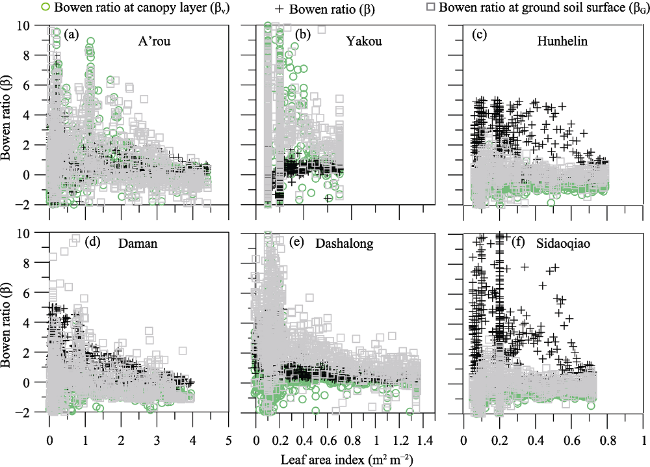
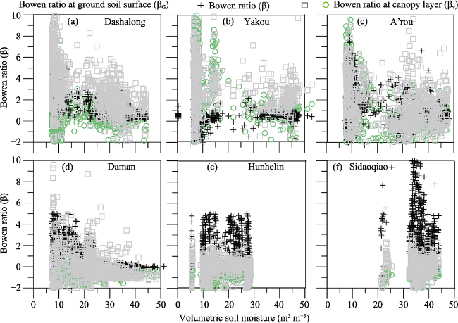
3.4 Relationship between leaf development, soil water dynamics and energy flux partitioning
The dependence of ecosystem energy partitioning on LAI was shown in Figure 5 for sites of Dashalong, Yakou, A’rou, Daman, Hunhelin and Sidaoqiao. The relationship between daily mean volumetric soil moisture and Bowen ratio for each site was shown in Figure 6. There was a trend of convergence of Bowen ratio with both development of LAI and increase of soil moisture. The amplitude of convergence of Bowen ratio was more obvious with the development of LAI compared with increase of soil moisture, suggesting that the leaf development dominates the energy partition for the six ecosystems in the HRB. The results indicate that leaf development explains the seasonality of Bowen ratio and dominates the lET flux for the six ecosystems.
Figure 6 Relationship between daily mean volumetric soil moisture and Bowen ratio for the Heihe River Basin from 2014 to 2016
4 Discussion
4.1 Energy partitioning with separation of plant and soil surface
Bowen ratio, generally measured by Bowen ratio system or EC system, failed to separate total energy flux into soil and vegetation surface by traditional methods. Two-source model is a useful tool for integrating the energy/water processes with separate lE (HG) and lT (HV) in terrestrial ecosystems and has the advantage of enabling process-based assessment of energy partitioning between soil and vegetation surface. Although previous studies used other methods to partition energy flux at vineyard (Zhao et al., 2017), there are several advantages of our modeling approach. First, the model treats the radiation/energy balance properly in both vegetative canopy and at the ground surface with interaction between them, enabling us to estimate all the total energy balance components, which can be comparable with measured Bowen ratio for model validation and to separate the Bowen ratio between canopy and soil surface. In this way, we can assess qualitatively the role of soil and plant for ecosys-tem energy partitioning. The model is solved by Newton-Raphson iteration scheme to simply, stably and rapidly estimate leaf temperature (TL) and ground soil temperature (TG) without directional radiometric temperature. The estimated TL and TG can be useful for model validation and reconstructing the surface temperature of various ecosystems. Second, changes of surface albedo with leaf development, and stomatal control of latent heat flux by transpiration including its dependence on soil moisture are explicitly considered in the model. Finally, the differences of ecohydrological (e.g. root depth, maximum and minimum stomatal resistance, canopy structure) and soil property (e.g. soil saturation moisture) among alpine vegetation, agriculture ecosystem and riparian ecosystem were taken into consideration in the model. However, there also exist many uncertainties for energy partitioning with separation of plant and soil surface, which still need to be improved. In reality, the terrestrial ecosystems have complex land surface (e.g. snow cover in winter). The amount of LAI ranged from close to nil after snow melt, up to 3-5 m2 m-2 (Figure 3). During periods of snow cover almost all shortwave radiation was reflected by the white surface and midday means of the albedo (α) varied between 0.7-0.8 with observed dataset. In this study, the land was mainly covered by vegetation and soil, this assumption accounted for errors of energy partitioning with separation of plant and soil surface. The values of some parameters (e.g. rst_min, rst_max, αv and αg) were fixed throughout the periods investigated; water source of plant of each ecosystems was fixed throughout the periods investigated which may change seasonally or yearly. Those uncertainties may result in errors for energy partitioning.
4.2 Biophysical control of seasonal convergence of energy flux partitioning
Previous studies have shown biophysical control on energy partitioning of temperate mountain grassland (e.g. Hammerle et al., 2008) and vineyard (Zhao et al., 2017). Our results support this view for the typical ecosystems within the HRB. Strictly speaking, the daily and seasonal variations of β, βV and βG are mainly controlled by LAI through changes of surface albedo and regulating permittivity. The surface albedo increased with increased LAI, and changing surface albedo was mainly controlled by LAI during growing seasons for the six ecosystems. The permittivity decreased with increased LAI, and controlled solar radiation partitioning between soil and plant surface. Also, the daily or seasonal variations of β, βV and βG are primarily controlled by LAI through regulating canopy conductance. With leaf development, more and more water was lost through plant transpiration with increased canopy conductance. Besides, the present study suggests soil moisture variation has impact on β, βV and βG (Figure 6), which indicate that soil water is primarily controlled energy partitioning through regulating canopy conductance during the drought period.
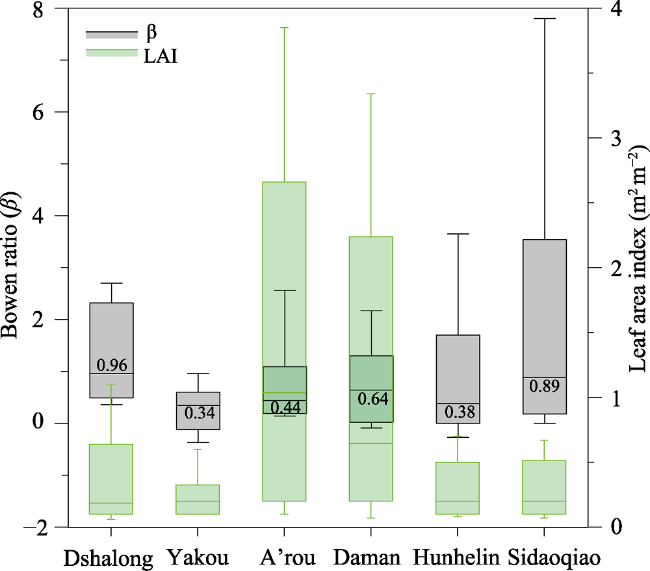
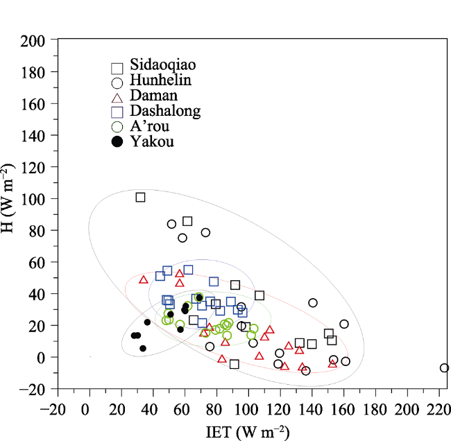
Strong biophysical controls of β were commonly found in previous studies. However, the relationship or its functional form varied among sites. Our results also showed different relationships for the typical ecosystems within the HRB. Figure 7 shows the statistics of LAI and β for the six ecosystems. Although there is close relationship between LAI and β, but differences are still shown in sensitivities of LAI to regulation of β. We find the riparian forest ecosystem (Sidaoqiao) has higher sensitivity to regulating energy partitioning, followed by alpine desert ecosystem characterized by smaller variations of LAI (Figure 7). From Figure 8, we find there are larger fluctuations of β for ecosystems of riparian forest and agriculture ecosystem, but conserve day to day fluctuations for A’rou (alpine meadow ecosystem), Dashalong (alpine swamp meadow ecosystem) and Yakou (alpine desert eco-system) during the growing season (from May to September). The di-vergent changes of β among the ecosystems are probably influenced by climate (Ta, and VPD) and soil water. The ecosystems in upper, middle and downstream show similar behavior of energy partitioning. Because the larger and rapid changes of VPD regulated by groundwater fluctuations of riparian ecosystems in downstream, the monthly fluctuations of lET, H and β are the largest. On the contrary, for alpine ecosystems, the monthly fluctuations of lET, H and β are the smallest because of the smallest changes of air temperature, which is the dominant factor for energy parti-tioning. Daman (agriculture ecosys-tem) has larger changes in LAI, but a smaller change in Bowen ratio, which is mainly due to the regulation of irri- gation and soil water dynamics. The ecosystems in upstream show subtle difference, the smallest variations of H and β of Dashalong site which may be related by its largest heat storage as alpine swamp meadow ecosystem. The smallest values of H and lET of Yakou, followed by Dashalong and A’rou, corresponded their elevations. Hunhelin showed a lower value of β than Sidaoqiao, which can be explained by the ecohydrlogical difference of plants and the distance between the sites and river channel.
Figure 7 Box-Whisker plots, which show the minimum, maximum, median, lower quartile, and upper quartile, for Bowen ratio in the Heihe River Basin from 2014 to 2016
Figure 8 Average monthly sensible and latent heat flux (lET) for different ecosystems measured by eddy covariance. Dashed lines show Bowen ratio of 1 (β), including A’rou (alpine meadow ecosystem), Dashalong (alpine swamp meadow ecosystem), Yakou (alpine desert ecosystem), Daman (cropland ecosystem), Sidaoqiao (T.ramosissima ecosystem), and Hunelin (P.euphratica ecosystem) sites in the Heihe River Basin
5 Conclusions
Using eddy covariance flux measurements of sensible and latent heat, soil heat flux, combined with energy-balanced two-source model, energy partitioning was investigated across six typical ecosystems in the Heihe River Basin. Bowen ratio (β) among the six sites exhibited significant seasonal variations with smaller inter-annual fluctuations. All the ecosystems exhibit a “U-shaped” pattern, characterized by a smaller value of β in growing season, with a minimum value in July, and a daily fluctuation. During the growing season, average Bowen ratio was the highest for the alpine swamp meadow (0.60 ± 0.30), followed by the desert riparian forest Populus euphratica (0.47 ± 0.72), the alpine desert (0.46 ± 0.10), the Tamarix ramosissima desert riparian shrub ecosystem (0.33 ± 0.57), alpine meadow ecosystem (0.32 ± 0.17), and cropland ecosystem (0.27 ± 0.46). At the daily or seasonal timescales, LAI is the primary controlling factor, regulating both surface albedo, solar radiation permissively to soil surface and canopy resistance. Soil water is primarily controlled by energy partitioning through regulating canopy conductance during the drought period. The results of this study highlight a two-source model, which is a useful tool for integrating the energy/water processes with separate E (HG) and T (HV) in terrestrial ecosystems and has the advantage of enabling long-term assessment of energy partitioning between canopy and soil surface. The importance of biophysical control explains the convergence of seasonal and annual patterns of Bowen ratio for all the ecosystems, and the changes in Bowen ratio showed divergence among various ecosystems because of different physiological responses and vegetation growth to energy flow pathways (e.g. lE (HG) and lT (HV)) between canopy and soil surface.
Supporting Information for
Vegetation dynamics dominate the energy flux partitioning across typical ecosystem in Heihe River Basin: Observation with numerical modeling
WANG Pei, LI Xiaoyan, TONG Yaqin, HUANG Yongmei, YANG Xiaofan, WU Xiuchen
State Key Laboratory of Earth Surface Processes and Resource Ecology, Faculty of Geographical Science, Beijing Normal University, Beijing 100875, China
Introduction
This text S1 provides the main equations in two-source model used in this study and summary of parameters for each site.
Text S1
The important formulas and methods involved in the estimation of evapotranspiration and latent heat are as follows:
where RnV and HV is the net radiation (W m-2) and sensible heat flux (W m-2) from the vegetation canopy, T is the transpiration flux (kg m-2 s-1), fV is the permittivity of the vegetation canopy, αV is the albedo of the vegetation canopy, Sd is the downward shortwave radiation (W m-2), Ld is the downward longwave radiation (W m-2), σ is the Stefan-Boltzmann constant (=5.67$\times$108 W m-2 K-4), TG is the ground surface temperature (oC), TL is the leaf temperature (oC), RnG is the net radiation at the ground surface (W m-2), G is the ground heat flux (W m-2), HG is the sensible heat flux from the ground surface (W m-2), E is the evaporation flux (kg m-2 s-1) and αG is the albedo of the ground surface. Note that this model is not a patch model but a layer model (Lhomme and Chehbouni, 1999), so total flux per unit area is given as the sum of vegetation canopy and ground surface components, that is, Rn = RnV+ RnG, H=HV +HG and lET = l(E+ T).
The fV was given as a function of LAI as follows:
${{f}_{V}}=1-\tanh ({{C}_{LAI}}LAI)$
where CLAI is the empirical constant and can be revised according to the specific situation of different ecosystems in the study area. The αV and αG were assumed to be constant as 0.2 and 0.1, respectively.
The HV and HG can be given by the following bulk equations:
where qsat(TL) is the saturated specific humidity for the leaf temperature (kg kg-1), qsat(TG) is saturated specific humidity for the ground surface temperature (kg kg-1), qa is the air specific humidity (kg kg-1) as a function of Ta, ha and air pressure (P), raV is the aerodynamic resistance for vegetation canopy (s m-1), rc is the canopy (stomatal) resistance (s m-1), raG is the aerodynamic resistance for ground surface (s m-1), and rSS is the surface soil resistance (s m-1). rc=rst/LAIrst is leaf stomatal resistance, although there are many scholars have proposed rst parameterization in this two-source model using the following calculation:
where rst_min and rst_max are the minimum and maximum values, respectively, of leaf stomatal resistance (s m-1), according to the vegetation type in different ecosystem we set different rst_min according to previous study (Kelliher et al., 1993; Koetz et al., 2005; Nagler et al., 2004) and calculated use field observation of the maximum stomatal conductance by Li6400XTportable Photosynthesis Measurement System (LICOR, USA). In accordance with the same method to determine the empirical parameters: CSW = θ/θmax, θ is the volumetric soil water content (m3 m-3) in different ecosystems, we set them according to the measured soil moisture content, and Csd =25 W m-2. The rsoil was given as the function of θ with a power term (Sun, 1982):
where θs is saturated water content (m3 m‒3). Because the soil in most site of HRB is merely saturated, the θs was set as θmax. Empirical constants were derived by the trial and error methods to optimize the modeling simulation for energy flux (Table S1).
Table S1 List of input parameters in the two-source model for each site
Site
cLAI
rst_min
rst_max
λss
zss
zm
zh
albV
albG
A’rou
1
100
10000
0.4
1
1
1
0.2
0.1
Dashalong
1
100
10000
0.4
1
10
5
0.2
0.1
Yakou
1
100
10000
0.4
0.4
10
5
0.2
0.1
Daman
1
40
10000
0.4
0.8
4
5
0.2
0.1
Sidaoqiao
1
60
10000
0.4
0.8
10
10
0.2
0.1
Hunhelin
1
50
10000
0.4
1
28
28
0.2
0.1
In the present study, the Newton-Raphson (NR) iteration scheme was introduced to solve Equations (1) and (2) simultaneously for TL and TG, respectively. If measured values of Sd, Ld, u, Ta, ha, P, LAI, zv, Tsoil and θ were given, we get TL and TG to calculate all the energy/water fluxes. The NR scheme is a robust method used to obtain a numerical solution with a higher rate of convergence (Paniconi and Putti, 1994) and has been used for solving energy balance equations diagnostically (e.g., Yamanaka et al., 1997). Rearranging Equations (1) and (2) with x=TL and y = TG, we can define the following two functions:
Approximate solutions of x and y closer to true values can be obtained by computing the following repeatedly:
$\left( \begin{matrix} \Delta x \\ \Delta y \\\end{matrix} \right)={{\left( \begin{matrix} a & b \\ c & d \\\end{matrix} \right)}^{-1}}\left( \begin{matrix} -F \\ -G \\\end{matrix} \right)$,
where Δx = xi+1 - xi, Δy = yi+1 - yi, subscript i denotes iteration number, Rw is the gas constant for water vapor, and esat(xi) or esat(yi) is the saturation vapor pressure at a temperature xi or yi. This iteration was continued until absolute values of both Δx and Δy are less than 0.0001.
References
[1] Kelliher F M, Leuning R, Schulze E D, 1993. Evaporation and canopy characteristics of coniferous forests and grasslands. Oecologia, 95(2): 153-163.
[2] Koetz B, Baret F, Poilve H et al., 2005. Use of coupled canopy structure dynamic and radiative transfer models to estimate biophysical canopy characteristics. Remote Sensing of Environment, 95: 115-124.
[3] Lhomme J P, Chehbouni A, 1999. Comments on dual-source vegetation-atmosphere transfer models. Agricultural and Forest Meteorology, 94: 269-273.
[4] Nagler P, Glenn E, Thompson T et al., 2004. Leaf area index and Normalized Difference Vegetation Index as predictors of canopy characteristics and light interception by riparian species on the Lower Colorado River. Agricultural and Forest Meteorology, 116: 103-112.
[5] Paniconi C, Putti M, 1994. A comparison of Picard and Newton iteration in the numerical solution of multidimensional variably saturated flow problems. Water Resources Research, 30(12): 3357-3374.
[6] Sun S F, 1982. Moisture and heat transport in a soil layer forced by atmospheric conditions [D]. Mansfield: University of Connecticut.
[7] Yamanaka T, Takeda A, Sugita F, 1997. A modified surface-resistance approach for representing bare-soil evaporation: Wind-tunnel experiments under various atmospheric conditions. Water Resources Research, 33: 2117-2128.
AroraV , 2002. Modeling vegetation as a dynamic component in soil-vegetation-atmosphere transfer schemes and hydrological models. Reviews of Geophysics, 40(3): 3-1-3-26.
[2]
BurakowskiE, TawfikA, OuimetteAet al., 2018. The role of surface roughness, albedo, and Bowen ratio on ecosystem energy balance in the eastern United States. Agricultural & Forest Meteorology, 249:367-376.
[3]
Chapin et al., 2002. Principles of Terrestrial Ecosystem Ecology. New York: Springer.
[4]
ChengG, LiX, ZhaoWet al., 2014. Integrated study of the water-ecosystem-economy in the Heihe River Basin. National Science Review, 1:413-428.
[5]
Good SP, NooneD, BowenG , 2015. Hydrologic connectivity constrains partitioning of global terrestrial water fluxes. Science, 349:175.
[6]
HammerleA, HaslwanterA , 2008. Leaf area controls on energy partitioning of a temperate mountain grassland. Biogeosciences, 5(2):421-431.
[7]
JasechkoS, Sharp ZD, Gibson JJet al., 2013. Terrestrial water fluxes dominated by transpiration. Nature, 496:347.
[8]
LiuS, LiX, XuZ , et al., 2018. The Heihe Integrated Observatory Network: A basin-scale land surface processes observatory in China. Vadose Zone Journal, 17:180072. doi: 10.2136/vzj2018.04.0072.
[9]
LiuS, XuZ, WangWet al., 2011. A comparison of eddy-covariance and large aperture scintillometer measurements with respect to the energy balance closure problem. Hydrology and Earth System Sciences, 15:1291-1306.
[10]
LiuS, XuZ, ZhuZet al., 2013. Measurements of evapotranspiration from eddy-covariance systems and large aperture scintillometers in the Hai River Basin, China. Journal of Hydrology, 487:24-38.
[11]
Maxwell RM, Condon LE , 2016. Connections between groundwater flow and transpiration partitioning. Science, 353:377.
[12]
NingL, ZhanC, LuoYet al., 2019. A review of fully coupled atmosphere-hydrology simulations. Journal of Geographical Sciences, 29(3):465-479.
[13]
PanX, Liu YB, Fan XWet al., 2017. Two energy balance closure approaches: Applications and comparisons over an oasis-desert ecotone. Journal of Arid Land, 9(1):51-64.
[14]
Shuttleworth WJ, WallaceJ , 1985. Evaporation from sparse crops: An energy combination theory. Quarterly Journal of the Royal Meteorological Society, 111:839-855.
[15]
Takle ES , 2015. Agricultural meteorology and climatology. Encyclopedia of Atmospheric Sciences, 25(680):92-97.
[16]
WangP, Li XY, Huang YMet al., 2016. Numerical modeling the isotopic composition of evapotranspiration in an arid artificial oasis cropland ecosystem with high-frequency water vapor isotope measurement. Agricultural and Forest Meteorology, 230/231:79-88.
[17]
WangP, Li XY, WangLet al., 2018. Divergent evapotranspiration partition dynamics between shrubs and grasses in a shrub-encroached steppe ecosystem. New Phytologist, 219:1325-1337.
[18]
WangP, TsutomuY , 2014. Application of a two-source model for partitioning evapotranspiration and assessing its controls in temperate grasslands in central Japan. Ecohydrology, 7:345-353.
[19]
WangP, TsutomuY, Li XYet al., 2015. Partitioning evapotranspiration in a temperate grassland ecosystem: Numerical modeling with isotopic tracers. Agricultural and Forest Meteorology, 208:16-31.
[20]
WangP, YamanakaT, Li XYet al., 2018. A multiple time scale modeling investigation of leaf water isotope enrichment in a temperate grassland ecosystem. Ecological Research, 33(5):901-915.
[21]
WangQ, YangW, HuangJet al., 2017. Shrub encroachment effect on the evapotranspiration and its component: A numerical simulation study of a shrub encroachment grassland in Nei Mongol, China. Chinese Journal of Plant Ecology, 41(3):348-358. (in Chinese)
[22]
Willmott CJ, Ackleson SG, Davis REet al., 1985. Statistics for the evaluation and comparison of models. Journal of Geophysical Research, 90(C5):8995-9005.
[23]
XuZ, LiuS, LiXet al., 2013. Intercomparison of surface energy flux measurement systems used during the HiWATER-MUSOEXE. Journal of Geophysical Research: Atmospheres, 118:13140-13157.
ZhaoP, Zhang, LiSet al., 2017. Vineyard energy partitioning between canopy and soil surface: dynamics and biophysical controls. Journal of Hydrometeorology, 18(7):1809-1829.
