Spatial-temporal variability of the fluctuation of soil temperature in the Babao River Basin, Northwest China

  • NING Lixin 1, 2, 3 ,
  • CHENG Changxiu , 1, 2, 3, * ,
  • SHEN Shi 1, 2, 3
Expand
  • 1 State Key Laboratory of Earth Surface Processes and Resource Ecology, Beijing Normal University, Beijing 100875, China
  • 2 Key Laboratory of Environmental Change and Natural Disaster, Beijing Normal University, Beijing 100875, China
  • 3 Center for Geodata and Analysis, Faculty of Geographical Science, Beijing Normal University, Beijing 100875, China
*Cheng Changxiu (1973-), Professor, specialized in complex system research. E-mail:

Ning Lixin (1991-), specialized in disaster risk analysis. E-mail: ninglixin123@163.com

Received date: 2018-10-23

  Accepted date: 2019-02-28

  Online published: 2019-12-11

Supported by

National Key R&D Program of China(No.2017YFB0504102)

National Natural Science Foundation of China(No.41771537)

Copyright

Copyright reserved © 2019. Office of Journal of Geographical Sciences All articles published represent the opinions of the authors, and do not reflect the official policy of the Chinese Medical Association or the Editorial Board, unless this is clearly specified.

Abstract

The Babao River Basin is the “water tower” of the Heihe River Basin. The combination of vulnerable ecosystems and inhospitable natural environments substantially restricts the existence of humans and the sustainable development of society and environment in the Heihe River Basin. Soil temperature (ST) is a critical soil variable that could affect a series of physical, chemical and biological soil processes, which is the guarantee of water conservation and vegetation growth in this region. To measure the temporal variation and spatial pattern of ST fluctuation in the Babao River Basin, fluctuation of ST at various depths were analyzed with ST data at depths of 4, 10 and 20 cm using classical statistical methods and permutation entropy. The study results show the following: 1) There are variations of ST at different depths, although ST followed an obvious seasonal law. ST at shallower depths is higher than at deeper depths in summer, and vice versa in winter. The difference of ST between different depths is close to zero when ST is near 5℃ in March or -5℃ in September. 2) In spring, ST at the shallower depths becomes higher than at deeper depths as soon as ST is above -5℃; this is reversed in autumn when ST is below 5℃. ST at a soil depth of 4 cm is the first to change, followed by ST at 10 and 20 cm, and the time that ST reaches the same level is delayed for 10-15 days. In chilling and warming seasons, September and February are, respectively, the months when ST at various depths are similar. 3) The average PE values of ST for 17 sites at 4 cm are 0.765 in spring > 0.764 in summer > 0.735 in autumn > 0.723 in winter, which implies the complicated degree of fluctuations of ST. 4) For the variation of ST at different depths, it appears that Max, Ranges, Average and the Standard Deviation of ST decrease by depth increments in soil. Surface soil is more complicated because ST fluctuation at shallower depths is more pronounced and random. The average PE value of ST for 17 sites are 0.863 at a depth of 4 cm > 0.818 at 10 cm > 0.744 at 20 cm. 5) For the variation of ST at different elevations, it appears that Max, Ranges, Average, Standard Deviation and ST fluctuation decrease with increasing elevation at the same soil depth. And with the increase of elevation, the decrease rates of Max, Range, Average, Standard Deviation at 4 cm are -0.89℃/100 m, -0.94℃/100 m, -0.43℃/100 m, and -0.25℃/100 m, respectively. In addition, this correlation decreased with the increase of soil depth. 6) Significant correlation between PE values of ST at depths of 4, 10 and 20 cm can easily be found. This finding implies that temperature can easily be transmitted within soil at depths between 4 and 20 cm. 7) For the variation of ST on shady slope and sunny slope sides, it appears that the PE values of ST at 4, 10 and 20 cm for 8 sites located on shady slope side are 0.868, 0.824 and 0.776, respectively, whereas they are 0.858, 0.810 and 0.716 for 9 sites located on sunny slope side.

Cite this article

NING Lixin , CHENG Changxiu , SHEN Shi . Spatial-temporal variability of the fluctuation of soil temperature in the Babao River Basin, Northwest China[J]. Journal of Geographical Sciences, 2019 , 29(9) : 1475 -1490 . DOI: 10.1007/s11442-019-1672-4

1 Introduction

The pedosphere is the most active and vital layer of the surface of the Earth (NRC, 2001). It is not only a core element that combines the atmosphere, hydrosphere, biosphere and lithosphere but is also an important nexus that controls the flow and transfer of material, energy and information. Moreover, soil is a material base essential for the existence and development of life on our planet (Chen et al., 2013). Soil provides food and energy for humans and plays an irreplaceable role in the regulation of the material cycle, maintenance of the ecological balance and protection of biodiversity (Karlen et al., 1997). Despite its role as the biogeochemical engine to support life on Earth, soil can also have major effects on society, economies, spirit, and culture (Robinson et al., 2012). With the growth of the global population and the development of the global economy, the global demand for fresh water and healthy food will increase by 100% and 50%, respectively, in the next 40 years (Godfray et al., 2010; Banwart et al., 2011). As a result, soil is facing a new set of intersecting challenges. Therefore, the demand for protecting soil, which is a limited resource, becomes increasingly urgent. To increase attention paid to the soil resource, the 68th United Nation General Assembly in 2013 declared December 5th of every year to be World Soil Day and 2015 as the International Soil Year. In addition, the “Global Soil Partnership” was launched by the Food and Agriculture Organization of the United Nations in 2012 (Montanarella and Vargas, 2012).
Soil temperature (ST) is one of the critical variables that affect a series of physical, chemical and biological processes within the soil. ST determines the quality of soil (Park et al., 2011) and thus influences the utilization of soil resources and the growth of plants (Kang et al., 2000) because the ideal ST band for plant growth is notably narrow, and plant root structure is inherently more sensitive to excessive temperature variations (Araghi et al., 2017). During the past decades, there have been many studies on the temporal pattern (Araghi et al., 2017), spatial pattern (Hu and Feng, 2003), and prediction of ST (Hengl et al., 2004). The above-mentioned studies on ST were mostly conducted using classical statistical methods. For instance, the Mann-Kendall method is used to analyze the significant differences of ST in different seasons, the average value and Coefficient of Variation are used to analyze the spatial variation of ST, and descriptive statistical methods are used to analyze temporal variations of ST. While the atmospheric system is a complex, nonlinear dynamical system (Liu et al., 2011), the time series of ST is non-stationary. As a result, there are problems in using classical statistical methods to analyze ST series.
With the development of science and improvement of the human cognitive level, complexity science has been gradually recognized as a new inter-discipline. The paradigm of complexity science has been gradually established (Liu et al., 2007; Dozier, 2011), and a wave of research regarding complexity science has arisen worldwide (Liu et al., 2007; Dozier, 2011). Under these conditions, the complexity research method has been generated, and the method has often been used advantageously to find laws that have proven impossible for the classical statistical method to find (Ludescher et al., 2016; Pele et al., 2017). For example, the Hurst exponent has been calculated to describe the long-range correlation of events (Gao et al., 2006; Gao et al., 2010), power spectra have been used to analyze periodic characteristics of events (Kanafi and Tuononen, 2017), and Information Theory has been used to quantify the uncertainty of events (Gao et al., 2013). Several scholars have used theories and methods of complexity science to analyze geographical phenomena and problems (Lin et al., 2007). Permutation entropy (PE) is a measure of the complexity of a dynamic system based on the comparison of neighboring values (Bandt and Pompe, 2002; Ning et al., 2018). It is a method used to describe the randomness or unpredictability of time series (Li and Li, 2017) and has been widely used to analyze the economy (Hou et al., 2017), instrument stability (Toomey and Kane, 2014), and the diagnosis of physical fitness (Gao et al., 2012; Kalpakis et al., 2015). Additionally, the method has been successfully used to analyze geographical phenomena (Stosic et al., 2016).
The Heihe River Basin is a typical inland river basin with an arid climate in Northwest China. The combination of vulnerable ecosystem, severe natural environment and scarcity of water resources substantially restricts social and economic development in this area (Li et al., 2009). The Babao River Basin, upstream of the Heihe River Basin, is the main water resource of the Heihe River. As the “water tower” to maintain the balance of water in the area, the condition of its ecosystem directly affects the existence of humans and the development of the economy (Song et al., 2017). In addition, it is related to the sustainable development of economy, society, and ecology in the middle and lower reaches of the Heihe River. Soil, an important part of the eco-environment, is the guarantee of water conservation and vegetation growth in this region. In this study, classical statistical methods and complexity methods (permutation entropy) are used to analyze the temporal and spatial variation of fluctuations of ST at different depths over the Babao River Basin. The relationship between fluctuation and altitude are also discussed. The research can help people to theoretically understand the nonlinear dynamic mechanisms of soil systems and to develop new soil models in practical applications. Moreover, this comprehensive analysis of temporal and spatial variation in ST fluctuations can help to elucidate the regional characteristics and guide local ecological construction. The main objective of this study is to help people protect and use land resources according to local ecosystem conditions to ensure the safety of land and water resources and maintain regional sustainable development.

2 Materials and methods

2.1 Study area

The study area in the Babao River Basin is the upstream of the Heihe River (Figure 1). The Babao River Basin, lying approximately between 37°43'15”N-38°18°24”N and 100°00'35”E -101°09'04”E, covers a total area of 2450 km2 in Qinghai Province (Shen et al., 2018). This area is characterized by scant precipitation, strong evaporation, frequent winds, and long sunshine hours. Located between two mountains with an elevation ranging from 2600 m to 5000 m, this basin is a typical intermontane basin generally characterized as having a semiarid and alpine cold climate (Ge et al., 2015), with an annual average precipitation of 400 mm (Zhang et al., 2018). According to the meteorological data recorded from 1990 to 2009, the mean air temperature was -4.2℃. Both precipitation and temperature vary significantly with elevation due to large elevation differences and steep topography (Qi and Luo, 2007). Mountain forest and grassland in the basin are the predominant vegetation types, and clear boundary lines between various landscapes exist with elevation. Glacial and snow-covered zones are widely distributed. The lower band of permafrost is between elevations of 3650 m and 3700 m (Kang et al., 2017).
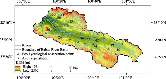
Figure 1 Location of the study area and the observation sites in the Babao River Basin

2.2 Data

To characterize eco-hydrological processes at the basin scale, an eco-hydrological wireless sensor network (EHWSN) was installed in the Heihe River Basin, supported by the Heihe Watershed Allied Telemetry Experimental Research (HiWATER) project. The ST dataset (Jin et al., 2014; Kang et al., 2015) acquired by ENWSN includes ST at depths of 4, 10, 20 cm at 17 observation sites (Figure 1) because others have insufficient data. The elevations of the 17 observation sites change from 3045 m (site 26) to 3843 m (site 45). Eight of the 17 sites are located in shrub area, three of the 17 sites are located in grassland area, and six sites are located in meadow area. Meanwhile, eight of the 17 sites are located on the sunny slope of the basin, and night sites are located on the shady slope of the basin. In summary, these 17 sites are evenly distributed throughout the basin. To ensure the integrity and comparability of ST, the time period selected for this study was from September 1, 2013 to August 31, 2014. Daily average ST at intervals of 10 min was calculated for the season when ST was observed. Other datasets were also needed, such as DEMs, the boundary of the Babao River Basin, and the boundary of the Heihe River Basin (version 2010).

2.3 Permutation entropy

Permutation entropy (PE) is a natural complexity measure for time series. The advantages of PE are its robustness, simplicity and fast calculation (Bandt and Pompe, 2002). In addition to its use to analyze the complexity of heart and brain data to distinguish healthy and sick subjects (Schwartz et al., 2004; Pardo-Igúzquiza and Rodríguez-Tovar, 2005), such a method has been successfully used to measure climate complexity (Stosic et al., 2016). The calculation process is as follows:
For a scalar time series$\left\{ x\left( i \right),i=1,2,\cdots \right\}$, an m- is first reconstructed:
$X\text{i}=\left\{ x\left( i \right),x\left( i+L \right),x\left( i+(m-1 \right)L) \right\}$
where m is called the embedding dimension and L the delay time. Here, m=5, L=1.
Next, the m number of real values \[X\text{i}=\left\{ x\left( i \right),x\left( i+L \right),x\left( i+(m-1 \right)L) \right\}\] can be arranged in an increasing order:
$x\left( i+\left( j\text{1}-1 \right)L \right)\le x\left( i+\left( j\text{2}-1 \right)L \right)\le \cdots \le x\left( i+\left( j\text{m}-1 \right)L \right)$
where j is a new series according to the previous processing.
When an equality occurs, e.g., $x\left( i+\left( j\text{i1}-1 \right)L \right)=x\left( i+\left( j\text{i2}-1 \right)L \right)$, we order the x according to their corresponding j. If ji1< ji2, we write $x\left( i+\left( ji\text{1}-1 \right)L \right)\le x\left( i+\left( ji\text{2}-1 \right)L \right)$
Therefore, any vector Xi is uniquely mapped onto {j1, j2, …, jm}, which is one of the m! permutations. When each permutation is considered as a symbol, then Xi is represented by a symbol sequence. The number of distinct symbols can at most be m!.
Let P1, P2, …, Pk represent the probability distribution for the distinct symbols, where km!. Thus, PE is defined as
$PE=-\underset{j=1}{\overset{k}{\mathop \sum }}\,Pj\text{ }\ln Pj$
The maximum of PE (m) is ln(m!), and it is convenient to work with:
$0\le \text{PE}=PE\left( m \right)/\text{ln}\left( m! \right)\le 1$
Therefore, PE gives a measure of the departure of the time series under study from a completely random series. Here, 0<PE<1, and if PE = 1, the time series is completely random. The smaller the value of PE, the more regular the time series. More details and a simple example of PE can be found in (Riedl et al., 2013).

3 Results

3.1 Classical statistical methods of analysis for ST

3.1.1 Temporal variations of ST
Site 33 is selected as an example to describe temporal variations of ST at different depths (Figure 2). The horizontal axis represents time, and the vertical axis represents the water level.
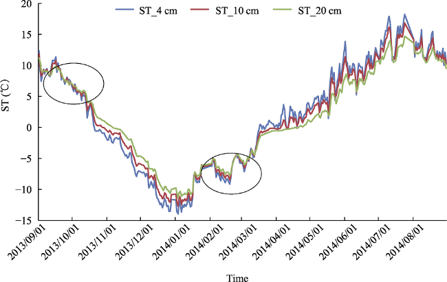
Figure 2 Temporal variation of ST (site 33) in the Babao River Basin
In general, variations of ST at depths of 4, 10 and 20 cm within a year display similar periodical patterns with a single peak or a cosine trend. STs in July and August were the highest, and later decreased until January, which was the lowest within a year. After January, ST at depths of 4, 10, and 20 cm experienced a significant increase until July.
The annual variation of ST at different depths was also slightly different. ST at a depth of 4 cm in August was higher than 20 cm, and ST at a depth of 10 cm is intermediate (Figure 2). The average STs at depths of 4, 10 and 20 cm in August were 12.48℃, 12.10℃ and 11.44℃, respectively. Additionally, ST at varies depths is basically similar in September, which can be observed in the first circle. In contrast, starting in October (ST is below 5℃), ST at deeper depths was higher than at shallower depths; this lasted until February, and the maximum difference occurred in December. The average STs at depths of 4, 10 and 20 cm in December were -10.36℃, -9.10℃ and -7.78℃, respectively. ST at various depths is basically the same in February, which can be observed in the second circle. Nonetheless, ST at shallower depths was higher than at deeper depths starting in March (ST was above -5℃).
It is also interesting that the time that ST changed to 0℃ at different depths is not the same, and a certain regularity is obvious. In the second half of the year, when ST is declining, ST at 4 cm first changes to 0℃, followed by 10 and 20 cm at an interval of approximately 7 days. In the first half of the year, when ST is rising, ST at 4 cm first rose to 0℃, followed by 10 and 20 cm, and the interval is approximately 17 days. Generally, change of ST at deeper soil depth lags behind change at shallower depth.
3.1.2 Spatial patterns of ST
ST observations at soil depths of 4, 10 and 20 cm at 17 sites in the Babao River Basin were collected to calculate classical statistical values at different depths, such as Max, Min, Range, Average, and Standard Deviation. In Table 1, some of the descriptive statistical values for ST at various depths are presented.
Table 1 List of stations used in this study
In general, relative to all stations, Max, Range, Average and Standard Deviation of ST decreased by increments of depths in the soil, and the highest value occurs at shallow depth, whereas the opposite occurs for Min. Taking site 33 as an example, ST Max values at depths of 4, 10 and 20 cm during the study period are 18.55℃, 16.91℃ and 14.84℃, respectively, compared with values of Min of -13.96℃, -12.71℃ and -11.41℃, respectively. The Average values are 1.91℃, 1.92℃ and 1.75℃, respectively.
To analyze the relationship between elevation and the classical statistical values, Pearson Correlation Coefficients were calculated by SPSS software. As seen in Table 2, there is a significant negative correlation between elevation and Max, Range, Average and Standard Deviation at depths of 4 cm, although not for Min. Statistically, with the increase of elevation, the decrease rates of Max, Range, Average, Standard Deviation at 4 cm are -0.89℃/100 m, -0.94℃/100 m, -0.43℃/100 m, and -0.25℃/100 m, respectively. In addition, this correlation decreased with the increase of soil depth, especially Range and Standard Deviation.
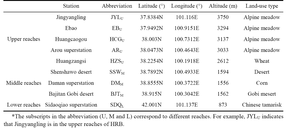
Table 2 Correlation between elevation and classical statistics of ST at different depths in the Babao River Basin
Soil depth Max Min Range Average Standard deviation
ST_4 cm -0.814** 0.057 -0.634** -0.648** -0.646**
ST_10 cm -0.757** -0.229 -0.396 -0.695** -0.490*
ST_20 cm -0.792** -0.343 -0.311 -0.749** -0.439*

** Correlation is significant at the 0.01 level (2-tailed)

*. Correlation is significant at the 0.05 level (2-tailed).

3.2 ST fluctuation

3.2.1 Temporal variation of ST fluctuation
The PE method was applied to the seasonal ST at different sites to determine the temporal variations of ST fluctuation (Table 3). Periods from March to May, from June to August, from September to November and from December to February were selected as spring, summer, autumn, and winter, respectively. Correlation analysis between the PE values and elevations was applied with the help of SPSS, and the correlation coefficients are given in the last line.
Table 3 PE values in different seasons for all sites and their correlations with elevation (4 cm depth) in the Babao River Basin
Site Elevation Spring Summer Autumn Winter
26 3045 0.786 0.795 0.813 0.729
30 3091 0.746 0.788 0.692 0.745
33 3335 0.779 0.778 0.775 0.800
34 3356 0.750 0.767 0.779 0.761
42 3413 0.752 0.758 0.755 0.774
29 3414 0.778 0.748 0.759 0.721
13 3462 0.751 0.772 0.749 0.693
49 3478 0.799 0.768 0.780 0.763
10 3484 0.757 0.764 0.751 0.707
47 3515 0.791 0.759 0.798 0.772
20 3538 0.723 0.746 0.761 0.756
41 3635 0.764 0.785 0.671 0.641
12 3766 0.744 0.773 0.694 0.692
16 3792 0.775 0.739 0.690 0.766
24 3813 0.796 0.813 0.770 0.610
39 3829 0.760 0.752 0.624 0.726
45 3843 0.748 0.689 0.637 0.640
Average - 0.765 0.764 0.735 0.723
Correlation coefficient 1 -0.047 -0.406 -0.580* -0.488*

* Correlation is significant at the 0.01 level (2-tailed)

In general, ST fluctuations are clearly different in the Babao River Basin, and the correlations between elevation and PE vary with the season. The average PE value for 17 sites in spring was 0.765, which was the highest, followed by summer, autumn and winter, the average PE values of which were 0764, 0.735 and 0.723, respectively. This finding implies that fluctuations of ST in spring and summer are more complicated and the changes of ST are more irregular and random than in other seasons, whereas the reverse occurs in winter. An interesting occurrence can be observed that the minimum PE value of ST occurs in site 45, whose elevation is 3846 m, the highest of all sites, whereas the maximum PE value occurs in sites at lower elevations.
Separate analyses for each season indicated that there is a negative correlation between elevation and PE value of ST, whereas it varies with the seasons. The strongest correlation occurs in autumn (correlation coefficient of -0.580) followed by winter, and the correlation coefficients is -0.488. However, there is no significant correlation between elevation and PE in spring and summer.
3.2.2 Spatial patterns of ST fluctuation
PE was applied to the STs from September 1, 2013 to August 31, 2014 at different depths at different sites to determine spatial patterns of ST fluctuation (Table 4).
Table 4 PE values at different elevation in the Babao River Basin
Elevation Site PE (ST_4 cm) PE(ST_10 cm) PE (ST_20 cm)
3045 26 0.898 0.854 0.825
3091 30 0.869 0.837 0.789
3335 33 0.899 0.865 0.766
3356 34 0.881 0.811 0.705
3413 42 0.883 0.84 0.773
3414 29 0.861 0.811 0.755
3462 13 0.866 0.822 0.794
3478 49 0.859 0.823 0.746
3484 10 0.848 0.812 0.738
3515 47 0.903 0.833 0.792
3538 20 0.863 - 0.742
3635 41 0.825 0.749 0.613
3766 12 0.84 0.8 0.772
3792 16 0.87 0.817 0.691
3813 24 0.871 0.828 0.756
3829 39 0.824 0.762 0.722
3843 45 0.804 - 0.676
Average 0.863 0.818 0.744
The results showed that the PE value differences of ST at various depths are obvious. In general, PE of ST at a depth of 4 cm is the highest, close to 1, whereas it varies with elevation. This finding implies that the fluctuation of ST at 4 cm is more complicated and random than at other depths. A pronounced phenomenon can be observed is that the PE value varies with soil depth. The ST PE values at 10 cm at all sites are lower than PEs at 4 cm; the average values are 0.818 and 0.863, respectively. The PE values of ST at 20 cm at all sites are lower than at 10 cm; the difference is 0.074. This means that fluctuation of ST at upper depths is more complex and the change of ST is more irregular and random than at shallower depths.
Correlation analysis between the PE values and elevations was applied with the help of SPSS, and the correlation coefficients are listed in Table 5.
Table 5 Correlation between PE and elevation at different depths in the Babao River Basin
Correlation coefficient Elevation PE (ST_4 cm) PE (ST_10 cm) PE (ST_20 cm)
Elevation 1 -0.629** -0.595* -0.556*
PE (ST_4 cm) - 1 0.889** 0.654**
PE (ST_10 cm) - - 1 0.755**
PE (ST_20 cm) - - - 1

**. Correlation is significant at the 0.01 level (2-tailed).

*. Correlation is significant at the 0.05 level (2-tailed).

It appears that significant negative correlation can be found between elevation and ST PE value at 4 cm with a correlation coefficient of -0.629. This finding suggests that PE of ST at this depth obviously decreased with the increase of elevation, that is, the fluctuation complexity of ST decreased. Further observations suggest that an increase in soil depth weakens the significant correlation between PE and elevation, which can be seen from the correlation coefficients between elevation and PE at 10 and 20 cm, -0.595 and -0.556, respectively.
A significant correlation between ST PE values at different depths can easily be found. Correlation coefficients between PE values at depths of 4 and 10 cm, 10 and 20 cm, and 4 and 20 cm are 0.889, 0.755 and 0.654, respectively. This implies that temperature can easily be transmitted within soil between depths of 4 and 20 cm.
The spatial distribution (Figure 3) of PE of ST at a depth of 4 cm in the Babao River Basin was mapped by means of Co-Kriging, and a significant correlation between PE and elevation was found.
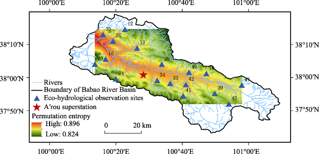
Figure 3 Spatial distribution of PE in the Babao River Basin
At the same time, the PE method was applied to the STs of different sites on both shady slope and sunny slope sides to determine the difference of ST fluctuation patterns at different areas (Table 6). There are eight observation sites located on shady slope side in the Babao River Basin, and night observation sites located on sunny slope side in the Babao River Basin. Here, the average PE value of ST at depths of 4, 10 and 20 cm are calculated, and the seasonal PE values of ST at a depth of 4 cm are calculated to analyze the seasonal difference of ST fluctuation.
Table 6 PE values of ST of different sites on shady slope and sunny slope sides in the Babao River Basin
Site PE
(ST_4 cm)
PE
(ST_10 cm)
PE
(ST_20 cm)
Spring
(4 cm)
Summer (4 cm) Autumn
(4 cm)
Winter
(4 cm)
Shady
slope
10 0.848 0.812 0.738 0.757 0.764 0.751 0.707
12 0.840 0.800 0.772 0.744 0.773 0.694 0.692
13 0.866 0.822 0.794 0.751 0.772 0.749 0.693
26 0.898 0.854 0.825 0.786 0.795 0.813 0.729
29 0.861 0.811 0.755 0.778 0.748 0.759 0.721
30 0.869 0.837 0.789 0.746 0.788 0.692 0.745
47 0.903 0.833 0.792 0.791 0.759 0.798 0.772
49 0.859 0.823 0.746 0.799 0.768 0.780 0.763
Average value 0.868 0.824 0.776 0.769 0.771 0.754 0.728
Sunny slope 16 0.870 0.817 0.691 0.775 0.739 0.690 0.766
20 0.863 - 0.742 0.723 0.746 0.761 0.756
24 0.871 0.828 0.756 0.796 0.813 0.770 0.610
33 0.899 0.865 0.766 0.779 0.778 0.775 0.800
34 0.881 0.811 0.705 0.750 0.767 0.779 0.761
39 0.824 0.762 0.722 0.760 0.752 0.624 0.726
41 0.825 0.749 0.613 0.764 0.785 0.671 0.641
42 0.883 0.840 0.773 0.752 0.758 0.755 0.774
45 0.804 - 0.676 0.748 0.689 0.637 0.640
Average value 0.858 0.810 0.716 0.761 0.759 0.718 0.719
The results showed that PE values of ST on shady slope side are all higher than that at sunny slope area. They are 0.868, 0.824, and 0.776 of ST at depths of 4, 10 and 20 cm, respectively, on shady slope side, and they are 0.858, 0.810, and 0.716 at depths of 4, 10 and 20 cm, respectively, on sunny slope side. Meanwhile, the analysis revealed that this is consistent in different seasons.

4 Discussion

The Babao River Basin, a typical inland river basin with semiarid and alpine cold climate, is the “water tower” of the Heihe River. The condition of its ecosystem directly affects the existence of humans and the development of the economy, society, and ecology of the entire the Heihe River Basin. Therefore, it is highly important for decision-makers to conduct ecological planning based on full consideration of vulnerable ecosystems and severe natural environments. What this research has achieved can help ecologists understand the temporal and spatial variations of ST from another perspective that is practically and theoretically important. Moreover, these findings can help decision makers to acquire more information regarding the Babao River Basin and take correct and effective protective measures to maintain sustainable development.
The temporal variation of ST is similar in shape to the shape of temporal variations of ST within a year at different depths. Cosine patterns of ST at various depths are clearly visible in Figure 3, which shows that STs in June and August are the highest within a year and ST is the lowest in December. This trend is basically consistent with the trend of solar radiation within a year because a change of solar radiation will directly affect the change of ST. Related research has also found a significant positive correlation between air temperature and ST (Islam et al., 2015), with a correlation coefficient above 0.95. Additionally, fluctuation of ST in spring and summer showed a much more complex pattern than ST in autumn, and winter. One of the key reasons is that the region has formed a unique atmospheric circulation system in the arid climate background because of its special geographical location. Due to the variation of atmospheric circulation, it will not only be affected by the warm and humid air transported by the southeast monsoon in summer but also by air transported from the Indian Ocean (Lan et al., 2015). Precipitation data recorded by the A’rou superstation showed that total precipitation during the study period was 449.9 mm, whereas it was 403.1 mm in spring and summer, or 90.0%. Despite high temperature, it should be noted that more precipitation means the atmospheric system in the region is more unstable, more susceptible to change and easier to change. Precipitation is accompanied by a decrease of air temperature and an increase of soil moisture that will consequently lead to ST fluctuation.
With respect to the variation of ST at different depths, it appears that the ranges of ST decrease, and the amplitudes of cosine curves decrease with increasing soil depth. As mentioned in section 3.1, the ST at a depth of 4 cm changed severely, followed by STs at depths of 10 and 20 cm. As seen in Table 4, the surface soil system is a much more complicated system because the fluctuation of ST at shallower depth is more violent and random. Additionally, the time that STs at depths of 4, 10 and 20 cm reach the same level will be delayed by approximately 10-15 days. The process of heat flow between the soil surface and the deeper depths was responsible for this phenomenon. Physically, soil surface temperature is decided by solar radiation, and heat transfer will occur that results from differences of ST at various depths. Nonetheless, soil heat conduction in warming and chilling seasons is different. In the chilling season, the solar shortwave radiation that the soil surface accepts is less than the longwave radiation that the soil surface releases, so the temperature of surface soil obviously drops. After a certain amount of time, the ST at various depths is similar. Nonetheless, after this time, a temperature gradient is formed between the soil surface and deeper depths, and heat is thus gradually transferred from deeper depths to shallower depths. A similar behavior (but reversed) of soil heat conduction can be seen in the warming season. While the process of heat transfer occurs over a certain period, a hysteresis of temperature response occurs. Moreover, there is another interesting conclusion that deeper soil systems are less complicated systems, and certain stability exits when ST is changing. Mechanically, ST in a short period of time will be somewhat affected by not only elevation and topography but also precipitation, weather conditions, and human activities. Even though there is a significant correlation of ST between shallow and deep depths, which implies that ST at deeper depths will be affected by ST at shallower depths, ST at deeper depths is mainly affected by elevation, topography, climate and other environmental factors. Although the change of ST at deeper depth is not obviously affected by short-term factors, such as the weather condition in a day or a few days, it will respond only when the season changes.
With respect to variation of ST at different elevations, it appears that the range fluctuates in a complicated way, and the amplitude of the cosine curve of ST decreases with increasing elevation. This tendency can be attributed to local special ecological environments. There is a large variation in elevation in the Babao River Basin. Therefore, more solar radiation is reflected by soil at higher elevation because the air is thin; the soil will thus acquire less net radiation to raise the ST, which results in slight fluctuation of ST. In contrast, the heat preservation ability of a dense atmosphere is stronger in low elevation areas. Additionally, human activities may be another factor; there are fewer human activities in high elevation areas than in low elevation areas. All of the reasons mentioned above lead to a more complicated system of soil at lower elevations than at higher elevations, and the variation of ST is more regular. At the same time, the calculated PE value of ST at shady slope area and sunny slope area appears that ST fluctuation at shady slope area is much more complicated because the fluctuation of ST at such area is more violent and random. This is still closely related to the solar radiation.

5 Conclusions and prospects

5.1 Conclusions

This study acquired the required data of the average values of ST at depths of 4, 10 and 20 cm at the daily scale from September 1, 2013 to August 2014 at 17 observation sites in the Babao River Basin. Temporal variations and spatial patterns of ST were analyzed with the help of classical statistical methods and the complexity method. Additionally, the correlation between ST fluctuation and elevation is discussed. The results showed the following: 1) Variation of ST at depths of 4, 10 and 20 cm within a year followed a similar trend with a single peak or a cosine. ST in July and August was the highest and decreased until January, which was the lowest within a year. After January, ST at 4, 10 and 20 cm increases until July. 2) In spring, ST at the shallower depths becomes higher than at deeper depths as soon as ST is above -5℃; this is reversed in autumn when ST is below 5℃. ST at a soil depth of 4 cm is the first to change, followed by ST at 10 and 20 cm, and the time that ST reaches the same level is delayed for 10-15 days. In chilling and warming seasons, September and February are, respectively, the months when ST at various depths are similar. 3) The average PE value of ST for 17 sites at 4 cm are 0.765 in spring > 0.764 in summer > 0.735 in autumn > 0.723 in winter, which implies the complicated degree of fluctuations of ST. 4) For the variation of ST at different depths, it appears that Max, Ranges, Average and the Standard Deviation of ST decrease by depth increments in soil. Surface soil is more complicated because ST fluctuation at shallower depths is more pronounced and random. The average PE value of ST for 17 sites are 0.863 at 4 cm > 0.818 at 10 cm > 0.744 at 20 cm. 5) For the variation of ST at different elevations, it appears that Max, Ranges, Average, Standard Deviation and ST fluctuation decrease with increasing elevation at the same soil depth. And with the increase of elevation, the decrease rates of Max, Range, Average, Standard Deviation at 4 cm are -0.89℃/100 m, -0.94℃/100 m, -0.43℃/100 m, and -0.25℃/100 m, respectively. In addition, this correlation decreased with the increase of soil depth. 6) Significant correlation between PE values of ST at 4, 10 and 20 cm can easily be found. This finding implies that temperature can easily be transmitted within soil at depths between 4 and 20 cm. 7) For the variation of ST at shady slope area and sunny slope area, it appears that the PE value of ST at 4 cm, 10 and 20 cm for 8 sites located on shady slope side are 0.868, 0.824, and 0.776, respectively, whereas they are 0.858, 0.810, 0.716 at depths of 4, 10 and 20 cm for 9 sites located on sunny slope side.

5.2 Prospects

To measure the temporal variation and spatial pattern of ST, permutation entropy was calculated to quantify the fluctuations of ST at various depths and their correlation with elevation. Additionally, the complexity method can, to a certain extent, reduce the influence of vegetation cover, slope, and other surface attributes. This analysis has achieved various results that may provide supplementary guidance on regional ecological construction and sustainable development. However, there are still certain limitations that need to be considered in the future. 1) Only temporal and spatial variations of ST at depths of 4, 10 and 20 cm are analyzed, not ST at deeper depths. 2) ST, soil moisture, air temperature and precipitation are basically parameters to describe the interactions of the soil-atmosphere system, and there are close connections and feedbacks between them. Therefore, additional investigation to quantify the interactions between the four parameters should be considered in the future. 3) It is interesting to find that there is no significant correlation between fluctuation complexity and elevation in spring and summer, which implies that elevation is not the main factor affecting fluctuations of ST in this region. More factors, such as topography, slope, aspect, and canopy, may affect the fluctuations of ST. Clarifying these factors’ relationships warrants further research.
[1]
Araghi A, Mousavi-Baygi M, Adamowski J , 2017. Detecting soil temperature trends in Northeast Iran from 1993 to 2016. Soil and Tillage Research, 174:177-192.

[2]
Bandt C, Pompe B , 2002. Permutation entropy: A natural complexity measure for time series. Physical Review Letters, 88(17):174102.

[3]
Banwart S, Bernasconi S M, Bloem J et al., 2011. Soil processes and functions in critical zone observatories: Hypotheses and experimental design. Vadose Zone Journal, 10(3):974-987.

[4]
Chen Y, Wang H, Zhou J et al., 2013. Minimum data set for assessing soil quality in farmland of northeast China. Pedosphere, 23(5):564-576.

[5]
Dozier J , 2011. Mountain hydrology, snow color, and the fourth paradigm. Eos, Transactions American Geophysical Union, 92(43):373-374.

[6]
Gao J, Hu J, Tung W-W et al., 2006. Assessment of long-range correlation in time series: How to avoid pitfalls. Physical Review E, 73(1):016117.

[7]
Gao J, Hu J, Tung W-W , 2012. Entropy measures for biological signal analyses. Nonlinear Dynamics, 68(3):431-444.

[8]
Gao J, Liu F, Zhang J et al., 2013. Information entropy as a basic building block of complexity theory. Entropy, 15(9):3396-3418.

[9]
Gao J, Sultan H, Hu J et al., 2010. Denoising nonlinear time series by adaptive filtering and wavelet shrinkage: A comparison. IEEE Signal Processing Letters, 17(3):237-240.

[10]
Ge Y, Wang J, Heuvelink G et al., 2015. Sampling design optimization of a wireless sensor network for monitoring ecohydrological processes in the Babao River Basin, China. International Journal of Geographical Information Science, 29(1):92-110.

[11]
Godfray H C J, Beddington J R, Crute I R et al., 2010. Food security: The challenge of feeding 9 billion people. Science, 327(5967):812-818.

[12]
Heng L T, Heuvelink G B, Stein A , 2004. A generic framework for spatial prediction of soil variables based on regression-kriging. Geoderma, 120(1/2):75-93.

[13]
Hou Y, Liu F, Gao J et al., 2017. Characterizing complexity changes in chinese stock markets by permutation entropy. Entropy, 19(10):514.

[14]
Hu Q, Feng S , 2003. A daily soil temperature dataset and soil temperature climatology of the contiguous United States. Journal of Applied Meteorology, 42(8):1139-1156.

[15]
Islam K I, Khan A, Islam T , 2015. Correlation between atmospheric temperature and soil temperature: A case study for Dhaka, Bangladesh. Atmospheric and Climate Sciences, 5(3):200.

[16]
Jin R, Li X, Yan B et al., 2014. A nested ecohydrological wireless sensor network for capturing the surface heterogeneity in the midstream areas of the Heihe River Basin, China. IEEE Geoscience and Remote Sensing Letters, 11(11):2015-2019.

[17]
Kalpakis K, Yang S, Hu P F et al., 2015. Permutation entropy analysis of vital signs data for outcome prediction of patients with severe traumatic brain injury. Computers in Biology and Medicine, 56:167-174.

[18]
Kanafi M M, Tuononen A J , 2017. Top topography surface roughness power spectrum for pavement friction evaluation. Tribology International, 107:240-249.

[19]
Kang J, Jin R, Li X et al., 2015. HiWATER: WATERNET observation dataset in the upper reaches of the Heihe River Basin in 2014. Heihe Plan Science Data Center.

[20]
Kang J, Jin R, Li X et al., 2017. High spatio-temporal resolution mapping of soil moisture by integrating wireless sensor network observations and MODIS apparent thermal inertia in the Babao River Basin, China. Remote Sensing of Environment, 191:232-245.

[21]
Kang S, Kim S, Oh S et al., 2000. Predicting spatial and temporal patterns of soil temperature based on topography, surface cover and air temperature. Forest Ecology and Management, 136(1-3):173-184.

[22]
Karlen D, Mausbach M J, Doran J et al., 1997. Soil quality: A concept, definition, and framework for evaluation (a guest editorial). Soil Science Society of America Journal, 61(1):4-10.

[23]
Lan Y, Ding H, Hu X , et al., 2015. The seasonal change characteristics of temperature, precipitation in the mountain areas of the Heihe River and Their Regional Differences. Mountain Research, 33(2):294-302.

[24]
Li X, Li C , 2017. Pretreatment and wavelength selection method for near-infrared spectra signal based on improved CEEMDAN Energy Entropy and Permutation Entropy. Entropy, 19(7):380.

[25]
Li X, Li X, Li Z et al., 2009. Watershed allied telemetry experimental research. Journal of Geophysical Research: Atmospheres, 114(D22).

[26]
Lin G, Chen X, Fu Z , 2007. Temporal-spatial diversities of long-range correlation for relative humidity over China. Physica A: Statistical Mechanics and Its Applications, 383(2):585-594.

[27]
Liu J, Dietz T, Carpenter S R et al., 2007. Complexity of coupled human and natural systems. Science, 317(5844):1513-1516.

[28]
Liu Y, Liu C, Wang D , 2011. Understanding atmospheric behaviour in terms of entropy: A review of applications of the second law of thermodynamics to meteorology. Entropy, 13(1):211-240.

[29]
Ludescher J, Bunde A, Franzke C L et al., 2016. Long-term persistence enhances uncertainty about anthropogenic warming of Antarctica. Climate Dynamics, 46(1/2):263-271.

[30]
Montanarella L, Vargas R , 2012. Global governance of soil resources as a necessary condition for sustainable development. Current Opinion in Environmental Sustainability, 4(5):559-564.

[31]
Ning L, Zhou Y, Yang J et al., 2018. Spatial-temporal variability of the fluctuation of water level in Poyang Lake basin, China. Open Geosciences, 10(1):940-953.

[32]
NRC, 2001. Basic Research Opportunities in Earth Science. Washington DC, USA: National Academies Press.

[33]
Pardo-Igúzquiza E, Rodríguez-Tovar F J , 2005. MAXENPER: A program for maximum entropy spectral estimation with assessment of statistical significance by the permutation test. Computers & Geosciences, 31(5):555-567.

[34]
Park S-G, Yi M-H, Shin H-T et al., 2011. Temporal change of soil animals of the stockpiled forest topsoil in relation to soil temperature and soil moisture. Journal of the Faculty of Agriculture, Kyushu University, 56(1):9-13.

[35]
Pele D T, Lazar E, Dufour A , 2017. Information entropy and measures of market risk. Entropy, 19(5):226.

[36]
Qi S, Luo F , 2007. Environmental degradation problems in the Heihe River Basin, Northwest China. Water and Environment Journal, 21(2):142-148.

[37]
Riedl M, Müller A, Wessel N , 2013. Practical considerations of permutation entropy. The European Physical Journal Special Topics, 222(2):249-262.

[38]
Robinson D, Hockley N, Dominati E et al., 2012. Natural capital, ecosystem services, and soil change: Why soil science must embrace an ecosystems approach. Vadose Zone Journal, 11(1).

[39]
Schwartz T U, Walczak R, Blobel G , 2004. Circular permutation as a tool to reduce surface entropy triggers crystallization of the signal recognition particle receptor β subunit. Protein Science, 13(10):2814-2818.

[40]
Shen S, Ye S, Cheng C et al., 2018. Persistence and corresponding time scales of soil moisture dynamics during summer in the Babao River Basin, Northwest China. Journal of Geophysical Research: Atmospheres, 123(17):8936-8948.

[41]
Song C, Yuan L, Yang X et al., 2017. Ecological-hydrological processes in arid environment: Past, present and future. Journal of Geographical Sciences, 27(12):1577-1594.

[42]
Stosic T, Telesca L, de Souza Ferreira D V et al., 2016. Investigating anthropically induced effects in streamflow dynamics by using permutation entropy and statistical complexity analysis: A case study. Journal of Hydrology, 540:1136-1145.

[43]
Toomey J, Kane D , 2014. Mapping the dynamic complexity of a semiconductor laser with optical feedback using permutation entropy. Optics Express, 22(2):1713-1725.

[44]
Zhang T, Shen S, Cheng C et al., 2018. Long range correlation analysis of soil temperature and moisture on A'rou Hillsides, the Babao River Basin. Journal of Geophysical Research: Atmospheres, 123(22):12606-612620.

Outlines

/