Stability and long-range correlation of air temperature in the Heihe River Basin

  • YANG Jing 1, 2, 3 ,
  • SU Kai 1, 2, 3 ,
  • YE Sijing , 1, 3, *
Expand
  • 1 State Key Laboratory of Earth Surface Processes and Resource Ecology, Beijing Normal University, Beijing 100875, China
  • 2 State Key Laboratory of Earth Surface Processes and Resource Ecology, Beijing Normal University, Beijing 100875, China
  • 3 State Key Laboratory of Earth Surface Processes and Resource Ecology, Beijing Normal University, Beijing 100875, China
*Ye Sijing (1988-), Assistant Professor, specialized in arable land quality evaluation and protection. E-mail:

Yang Jing (1989–), specialized in spatial-temporal analysis and disaster research. E-mail: yangj@mail.bnu.edu.cn

Received date: 2018-10-23

  Accepted date: 2019-02-20

  Online published: 2019-12-11

Supported by

Strategic Priority Research Program of the Chinese Academy of Sciences(No.XDA23100303)

Copyright

Copyright reserved © 2019. Office of Journal of Geographical Sciences All articles published represent the opinions of the authors, and do not reflect the official policy of the Chinese Medical Association or the Editorial Board, unless this is clearly specified.

Abstract

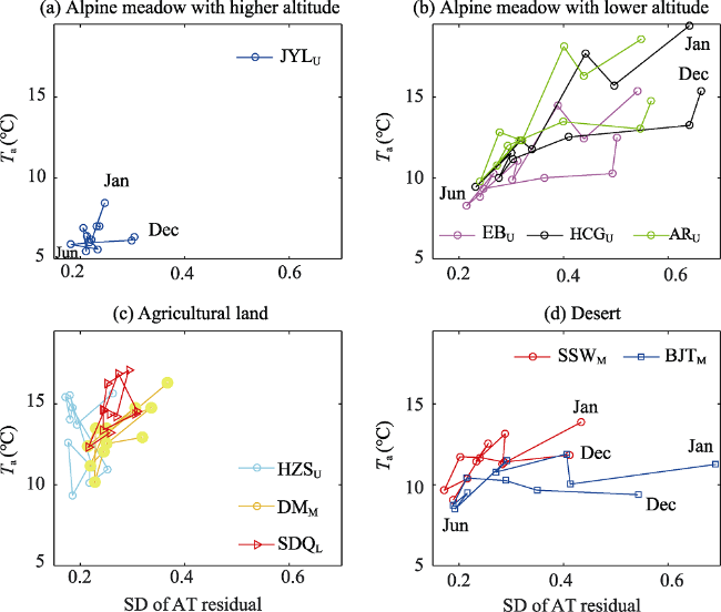
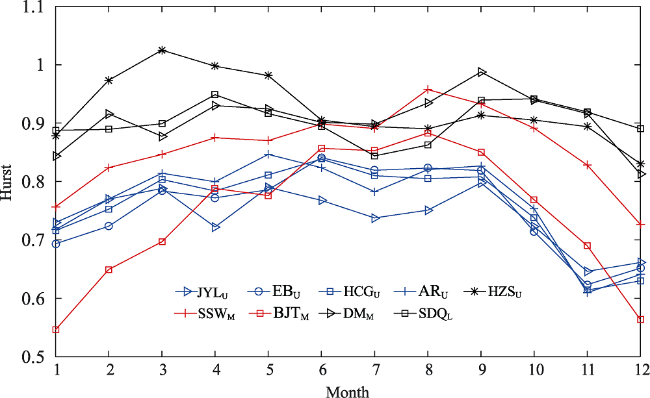
Air temperature (AT) is a subsystem of a complex climate. Long-range correlation (LRC) is an important feature of complexity. Our research attempt to evaluate AT’s complexity differences in different land-use types in the Heihe River Basin (HRB) based on the stability and LRC. The results show the following: (1) AT’s stability presents differences in different land-use types. In agricultural land, there is no obvious variation in the trend throughout the year. Whereas in a desert, the variation in the trend is obvious: the AT is more stable in summer than it is in winter, with Ta ranges of [8, 20]°C and SD of the AT residual ranges of [0.2, 0.7], respectively. Additionally, in mountainous areas, when the altitude is beyond a certain value, AT’s stability changes. (2) AT’s LRC presents differences in different land-use types. In agricultural land, the long-range correlation of AT is the most persistent throughout the year, showing the smallest difference between summer and winter, with the Hs range of [0.8, 1]. Vegetation could be an important factor. In a desert, the long-range correlation of AT is less persistent, showing the greatest difference between summer and winter, with the Hs range of [0.54, 0.96]. Solar insolation could be a dominant factor. In an alpine meadow, the long-range correlation of AT is the least persistent throughout the year, presenting a smaller difference between summer and winter, with the Hs range of [0.6, 0.85]. Altitude could be an important factor. (3) Usually, LRC is a combination of the Ta and SD of the AT residuals. A larger Ta and smaller SD of the AT residual would be conducive to a more persistent LRC, whereas a smaller Ta and larger SD of the AT residual would limit the persistence of LRC. A larger Ta and SD of the AT residual would create persistence to a degree between those of the first two cases, as would a smaller Ta and SD of the AT residual. In addition, the last two cases might show the same LRC.

Cite this article

YANG Jing , SU Kai , YE Sijing . Stability and long-range correlation of air temperature in the Heihe River Basin[J]. Journal of Geographical Sciences, 2019 , 29(9) : 1462 -1474 . DOI: 10.1007/s11442-019-1671-5

1 Introduction

Understanding the features and complexity of the air temperature (AT) has important implications for the development of ecosystems and climate change (Solomon et al., 2009). AT is arguably the most important component of climate (Zhang et al., 2003). It influences a broad range of ecosystem processes, including evapotranspiration, photosynthesis, decomposition, and carbon fixation (Running, 1987). Through these processes, AT affects vegetation dynamics and the distribution of biota. The spatial-temporal patterns of AT are particularly complex due to its interactions with components (Rind, 1999; Held, 2014) such as land cover, terrain, latitude, longitude, and vegetation (Cheng et al., 2008; Shao et al., 2012; Shiflett et al., 2017). Lorenz is the first to explicitly note the nonlinear dynamics of the atmosphere. Recently, Li (2014) also stressed that AT variance was spatially and temporally non-uniform. Xu et al. (2013) cited a few concepts and methods that have been used to reveal the complexity of the climate change process, with a focus on understanding the complexity of temperature dynamics in Xinjiang, China.
Diurnal temperature is one of the climate change characteristics. On the one hand, research on it would be helpful to know local climate (Pike et al., 2012), plant growth (Orlandini et al., 2006), local ecology (Armbruster et al., 2007), and earth surface processes. For example, diurnal temperature variation is an important index for urban heat island effect (Mathew et al., 2018); it has an impact on proanthocyanidin accumulation in grape skins (Cohen et al., 2012); and it is also used to estimate pore water fluid flux then further infer vertical groundwater-surface water exchange (Irvine et al., 2017). On the other hand, diurnal temperature could improve fine weather forecast. Yang et al. (2013) concluded general rules and seasonal characteristics of daily extreme temperature and the speed of temperature change in Beijing. This conclusion they proposed could serve as a background for fine weather forecast.
While considerable research was on AT complexity, they focused on decadal or century scale (Franzke, 2012; Gil-Alana, 2012; Østvand, 2014). Complexity research on AT’s time series at finer temporal scale should also be enhanced, and be expected to have some new discovery. Long-range correlation (LRC) is one of the complexity characteristics. It is distinguished from long-term range (Wu et al., 2013), which describes the amplitude and duration of evolution trends based on the autocorrelation structure of the time series (Michael, 2012). It is also known as long-range dependence, long memory, or long-range persistence (Shen et al., 2018). The LRC index reflects intensity of persistence or antipersistence (Zhang et al., 2018). This index on AT would show AT in certain time has much influence on future AT. It should be stressed that LRC evaluation depends on higher demand for data. The data should be high frequency and continuous.
Our research shows the AT’s complexity based on data at the scale of 10 minutes to evaluate complexity differences of different land-use types in Heihe River Basin (HRB) in 2014. AT’s complexity is detected by AT’s stability and LRC. Complexity in each month is calculated, and then the variations throughout the year are analyzed. Sections 2.1 and 2.2 show data description. Sections 2.3 and 2.4 show AT’s complexity. To describe the stability from different perspectives, monthly stability is qualitatively determined by the average daily temperature range (Ta) and standard deviation (SD) of the AT residual. Adaptive fractal analysis (AFA) is used to analyze AT’s LRC. Section 3 evaluates differences of AT’s complexity in different land-use types. Section 4 discusses the differences, and shows the relationship between AT’s stability and LRC. Section 5 gives some main conclusions.

2 Data and methods

2.1 Study area

The Heihe River Basin (HRB) is the second largest inland river basin in northwest China and central Eurasia, and it covers an area of approximately 128,000 km2, as shown in Figure 1. Administratively, the basin includes part of Qilian County in Qinghai Province, some counties and cities in Gansu Province, and part of Ejin Banner in Alxa League of Inner Mongolia.
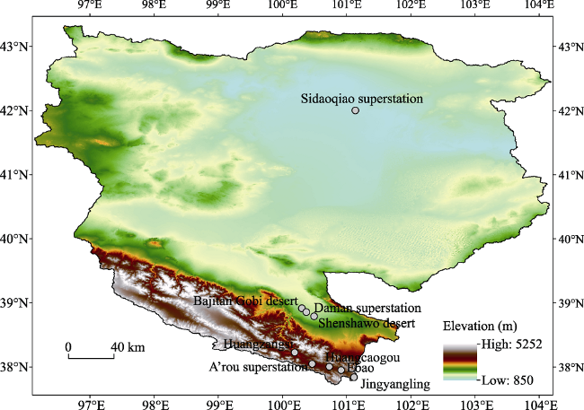
Figure 1 Location of stations in the Heihe River Basin in this study
Research on HRB will be of ecological significance. Because of HRB’s relatively abundant water resource (mean annual runoff is 37.3×10⁸ m3), the area is an important commodity grain base in northwest China. It covers diverse agricultural lands, including wheat, corn and Chinese tamarisk. However, it has recently experienced rapid socioeconomic development and an increase in population density (Song et al., 2017). Extensive exploitation of the water and land resources in the upper and middle parts of the basin has led to a sharp decrease in water resources in the lower reaches of the Heihe River. This has resulted in a severe deterioration of the eco-environment in the Ejin Banner Oasis, which is located in the downstream sections of the basin.
It is thus an optimal experimental area for understanding the variance of AT based on the geographical environment. Geographical differentiation is evident in the basin. From south to north, there are three major geomorphological units: the southern Qilian Mountains, the middle Hexi Corridor and the northern Alxa High-plain. The southern Qilian Mountains, with a remarkable vertical zonal gradient, is the water source area. The elevation of the area ranges from 2000 to 5500 m, and the mean annual precipitation increases from approximately 250 mm in the low-mountain or hilly zone to approximately 500 mm in the high-mountain zone. The middle Hexi Corridor is located between the Qilian Mountains and the Beishan Mountains. The elevation of the area decreases from > 2000 m to 1000 m, and the mean annual precipitation decreases from 250 mm to < 100 mm from south to north. The northern Alxa High-plain is mainly occupied by bare Gobi and Chinese Tamarisk, with a mean altitude of approximately 1000 m and a mean annual precipitation of < 50 mm.

2.2 Data

The dataset is from the “Heihe Watershed Allied Telemetry Experimental Research (HiWATER)” project (Liu et al., 2011; Kang et al., 2015). Data is recorded every 10 minutes, and 144 records are ensured every day. Each record corresponds to a moment. The AT data used in this research are obtained at a height of 5 m in 2014. AT data at a 5 m height are the most complete and cover most stations. Additionally, the data are concentrated in 2014.
This paper obtained AT data from nine stations, as shown in Figure 1 and Table 1. In addition to the completeness of data, different geographical environments were considered when selecting stations. These environments span a broad range of altitudes, latitudes and land-use types. The altitudes of the stations vary from 873 m to 3750 m, and the latitudes range from 37.8384° to 42.001°. The land-use types include alpine meadow, deserts and agricultural lands. From higher altitude to lower altitude and lower latitude to high latitude, the stations were JYLU, EBU, HCGU, ARU, HZSU, SSWM, DMM, BJTM and SDQL. Alpine meadow areas include JYLU, EBU, HCGU and ARU. Agricultural lands include HZSU, DMM and SDQL. Deserts include SSWM and BJTM. The subscript letter in the abbreviations (U, M and L) corresponds to different reaches. For example, JYLU means that the station is in the upper reaches of HRB.
Table 1 List of stations used in this study
Station Abbreviation Latitude (°) Longitude (°) Altitude (m) Land-use type
Upper reaches Jingyangling JYLU 37.8384N 101.116E 3750 Alpine meadow
Ebao EBU 37.9492N 100.9151E 3294 Alpine meadow
Huangcaogou HCGU 38.003N 100.7312E 3137 Alpine meadow
Arou superstation ARU 38.0473N 100.4643E 3033 Alpine meadow
Huangzangsi HZSU 38.2254N 100.1918E 2612 Wheat
Middle reaches Shenshawo desert SSWM 38.7892N 100.4933E 1594 Desert
Daman superstation DMM 38.8555N 100.3722E 1556 Corn
Bajitan Gobi desert BJTM 38.915N 100.3042E 1562 Gobi mesert
Lower reaches Sidaoqiao superstation SDQL 42.001N 101.137E 873 Chinese tamarisk

*The subscripts in the abbreviation (U, M and L) correspond to different reaches. For example, JYLU indicates that Jingyangling is in the upper reaches of HRB.

2.3 Qualitative estimation of AT’s stability

To describe the stability of AT from different perspectives, monthly stability is qualitatively estimated by the Ta and SD of the AT residuals. The monthly Ta is calculated using formula (1):
${{T}_{ai}}=\text{ }\!\!~\!\!\text{ }\frac{1}{n}\text{ }\!\!\Sigma\!\!\text{ }_{k=1}^{n}[\max \{{{T}_{i}}\left( k,j \right)\}-\min \{{{T}_{i}}\left( k,j \right)\}]\left( j=1,2\ldots ,144;\text{ }k=1,2\ldots ,n \right)$
Firstly, we calculated the daily temperature range, which is shown with $\max \{{{T}_{i}}\left( k,j \right)\}-$ $\min \{{{T}_{i}}\left( k,j \right)\}$in formula (1); then monthly Ta is average daily temperature range in a month. In the formula, i indicates which month is calculated and n is the number of days in month i and could be 28, 29, 30 or 31. k indicates which day is calculated in month i; j is a moment in a day, corresponding to one of 144 records; ${{T}_{i}}(k,j)$ is temperature at moment j, day k, and month i; and Tai is the average daily temperature range in month i.The monthly SD of AT residuals is also used to measure AT’s stability, as shown in Figure 2. First, the original AT series should be smoothed to get the trend, as shown by the red line in the figure. After many experiments, a period of 4 hours was considered an optimal interval for smoothing data to distinguish the stations’ stability. The smoothing method is the same as step (1) in AFA, which is introduced in the method of calculating LRC. Then, AT residuals are calculated as step (2) in AFA. Finally, the monthly SD is calculated.
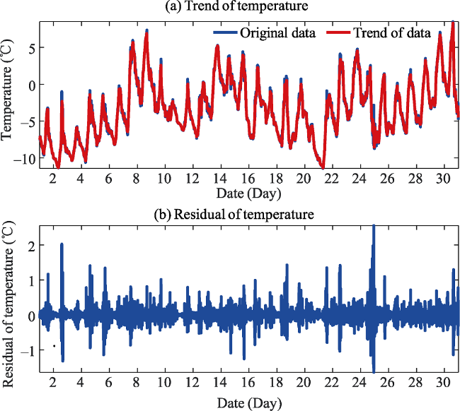
Figure 2 Residual of air temperature in Heihe River Basin from January 2014 to December 2014

2.4 Method for long-range correlation

After the qualitative estimation of AT’s stability, this paper quantifies the LRC of AT’s complexity. LRC is a way to express the “memory” or serial correlation in a time series. It is often called the Hurst exponent and is denoted as H. Usually, it is composed of 3 degrees: long-range correlation, negative long-range correlation and uncorrelated process. Anti-persistent and persistent processes contain structures that distinguish them from truly random sequences of data. 0.5 < H < 1 indicates a correlated process, or what is termed a persistent process. In this case, increases in the time series are likely to be followed by further increases, and decreases are likely to be followed by decreases. In addition, a finding of 0 < H < 0.5 indicates an anti-correlated or anti-persistent process, which means that increases in data series are likely to be followed by decreases (and decreases are likely to be followed by increases). H = 0.5 indicates that the process is random and that the data points are uncorrelated with each other.
In this paper, to effectively remove the trends of time series, adaptive fractal analysis (AFA) (Gao et al., 2019) is used to measure LRC. In some ways, it is similar to detrended fluctuation analysis (DFA). However, in addition to sharing many of the same advantages as DFA, AFA can deal with arbitrary and strong nonlinear trends by constructing overlapped sliding fitting windows (Gao et al., 2007; Riley et al., 2012). This method has been successfully used for chaos and fractal analysis of bio-signals (Guo et al., 2012). Its method of analysis is as follows:
(1) The first step in AFA is to identify a globally smooth trend that is created by patching together local polynomial fits to the time series. A global trend is a synthetic time series {vi}, i = 1, 2, ..., N, where N is length of the original time series. The fit to overlapping regions is created by taking a weighted combination of the fits of two adjacent regions. It ensures that the concatenation of local fits is smooth, according to formula (2) (Gao et al., 2007):
${{y}^{\left( c \right)}}\left( l \right)={{w}_{1}}{{y}^{\left( i \right)}}\left( l+n \right)+{{w}_{2}}{{y}^{\left( i+1 \right)}}\left( l \right)$
where ${{w}_{1}}=\left( 1-\frac{l-1}{n} \right)$ and ${{w}_{2}}=\frac{l-1}{n}$.
(2) The next step is to detrend the data by removing the global trend signal that was just created. Then, the residual of the original data is $\left\{ {{u}_{i}}-{{v}_{i}} \right\}$, where {ui} is the original data.
(3) The last step is to quantify the Hurst exponent, H, based on the relation between the variance of the magnitude of the residuals, F(w), and the window size, w, as formula (3) shows (Gao et al., 2007):
${{F}^{\left( 2 \right)}}\left( w \right)={{\left[ \frac{1}{n}\underset{i=1}{\overset{n}{\mathop \sum }}\,{{\left( {{u}_{i}}-{{v}_{i}} \right)}^{2}} \right]}^{1/2}}\tilde{\ }{{w}^{H}}$
H can be quantified through the slope (obtained using simple linear regression) of a linear relation in a plot of log2F(w) as a function of log2w.

3 Results

3.1 Qualitative estimation of AT’s stability

To analyze the differences in stability at each station, the monthly stability of these stations is now determined. Taking the SD of the AT residual as the x-axis and Ta as the y-axis, a month at a station corresponds to a point in the coordinate system. For every station, we may draw a direction line from January to December. The stability of each station is shown in Figure 3. AT presents a smaller range of fluctuation when the point is closer to the origin, which indicates that AT is more stable. In contrast, AT presents a larger fluctuation range when the point is farther from the origin, which indicates that AT is more unstable.
Figure 3 Stability of AT based on Ta and SD of AT Residual in Heihe River Basin from January 2014 to December 2014. Categories (a) and (b) are alpine meadow area, but the altitude of category (a) is higher than category (b); Category (c) is agricultural land area; and Category (d) is desert area.
Besides JYLU, AT’s stability presents differences in different land-use types. Nine stations are classed into four categories based on the lines of all stations: (1) AT of JYLU is stable throughout the year. Moreover, the difference in stability between summer and winter is the smallest at all stations. Both the Ta and SD of the AT residual are the lowest throughout the year, within 5℃ and 0.3, respectively. (2) AT of EBU, HCGU and ARU are more stable in summer than in winter. Moreover, the difference in stability between summer and winter is the greatest. Both the Ta and SD of the AT residual show obvious differences between winter and summer, with a range of [8, 20]℃ and [0.2,0.7], respectively. (3) There are no obvious variations in the trend of AT’s stability across the year in HZSU, DMM and SDQL. Their Ta ranges are greater than the SD of the AT residual, with ranges of [9, 18]℃ and [0.1, 0.4], respectively. (4) AT of SSWM and BJTM are more stable in summer than it is in winter. Moreover, the difference in stability between summer and winter is lower than that observed for category (b). In contrast to category (c), the range for the SD of the AT residual in these stations is greater than that of Ta, with [8, 14]℃ and [0.1, 0.7], respectively.

3.2 Quantified estimation of AT’s long-range correlation

This part quantitatively describes AT’s LRC. The variation of LRC with month is shown in Figure 4. Taking the month as the x-axis and the LRC as the y-axis, a month of a station’s data corresponds to a point in the coordinate system. For every station, we can draw a line from January to December.
Figure 4 Monthly LRC in each station in Heihe River Basin from January 2014 to December 2014. Different line colors correspond to different categories and to different land-use types. A black line is agriculture land, red is desert, and blue is alpine meadow.
There is a long-range correlation for all stations. The monthly H of each station is far greater than 0.5, and some of them even approach 1. This result indicates that ATs all behave as a persistent process, which means further increases (decreases) in AT are likely to occur in the next sampled moment. For example, in this paper, AT’s trend in the next 10 minutes is likely to be the same as that observed for the previous 10 minutes.
AT’s long-range correlation presents differences in different land-use types. According to the observed variation trend of LRC, the 9 stations are classified into three categories, which correspond to the different colors in Figure 4. The first category includes HZSU, DMM, and SDQL, which is shown with black lines. Their Hs are all greater than 0.8 and are among the highest in all categories throughout the year. Additionally, their fluctuations are not well pronounced. The second category includes SSWM and BJTM, which is shown with red lines. Although their values are more varied, they share a similar variance in monthly H. Their LRCs vary significantly between summer and winter. H is lower in winter months and higher in summer months, with ranges of [0.7, 0.96] and [0.54, 0.88], respectively. The last category includes JYLU, EBU, HCGU, and ARU, which is shown with blue lines. Their Hs are all lower than 0.85, and they generally remain lower throughout the year. In addition, they do not fluctuate significantly, except in November and December.

4 Discussion

4.1 Analysis on differences of AT’s stability

4.1.1 Impact of altitude on AT’s stability
First, altitude could be an important factor in AT’s stability, as categories (1) and (2) show. In mountainous areas, when the altitude lies beyond a certain value, the characteristics of AT’s stability could change. For categories (1) and (2), aside from their altitudes, their geographical environments are similar, including land-use type and latitudes. The altitude of JYLU is 3750 m in category (1). It is higher approximately 456 m than that of EBU, which is the highest station in category (2). Wang et al. (2011) stressed that altitude is an important factor in a climate system. When the altitude is beyond a certain value, the influence of altitude could be more significant than that of other climate components. This was similar to what Dobrowski et al. (2009) mentioned, i.e., when one component loses its explanatory power, the other is prevalent. In addition, owing to the high altitude, AT is closely coupled to atmospheric circulation. Thus, low-stature vegetation (Alpine Meadow) can effectively decouple from free convection (to create aerodynamic resistance to heat exchange) (Körner, 2007).
4.1.2 Impact of land-use type on AT’s stability
Land-use type has a good relation with AT’s stability. In the same land-use type, similar seasonal trends of Ta and SD of AT residuals could be observed. As shown in categories (3) and (4), the stations share the same land-use type, i.e., agricultural land or desert. In agricultural land, there is no obvious variation trend in AT’s stability across the year. Moreover, their Ta ranges are greater than those of the SD of AT residuals. In desert, the AT of the stations is more stable in summer than in winter. In contrast to agricultural land, the ranges of these stations’ SD of AT residuals are greater than the ranges of Ta. There is evidence indicating that AT affected land-use type by affecting phenology of organisms, the range and distribution of species, and the composition and dynamics of communities (Walther et al., 2002). Considering earth is a complex system with interactive components, land-use type could affect AT in turn. For example, rain falling on the Earth contributes to plant growth, and plant growth transpires the moisture back to the atmosphere during the process of growing. In addition, the atmospheric water vapor can form clouds, thereby affecting the solar radiation, which influences how plants grow (Rind, 1999).

4.2 Analysis on differences of AT’s long-range correlation

Land-use type has a good relation with AT’s LRC. In the three categories mentioned above, different categories correspond to different land-use types. They are agricultural land (category 1), desert (category 2) and alpine meadow (category 3).
In agricultural land, the long-range correlation of AT is the most persistent across the year in all land-use types. Additionally, it shows the least difference in LRC between summer and winter, possibly due to the influence of vegetation, which could have a positive influence on climate dynamics (Shiflett et al., 2017). These areas include wheat, corn and Chinese tamarisk. In summer, vegetation roots continually absorb water from the soil, and air maintains stable humidity levels. Dense vegetation reduces the wind speed, reduces airflow, and finally maintains AT’s stability. In winter, time lag could be an important factor for climate-vegetation interaction (Wu et al., 2015). Vegetation influences AT not only in real time but also for longer periods. In other words, this low level of complexity provides a suitable living environment for vegetation.
In deserts, the long-range correlation of AT is less persistent. Additionally, the greatest difference in LRC between summer and winter is observed in these stations. Solar insolation could be a dominant influencing factor. Because of the high H in summer, AT shows a more persistent process than it does in winter. This also means that AT’s variance trend in the next 10 minutes is more likely to be the same as in the previous 10 minutes in summer than it is in winter. Therefore, the AT in summer is less complex than winter. Solar radiation is strong in summer and weak in winter (Guo et al., 2012). Therefore, it could have a positive influence on AT in summer (Ricke et al., 2010; Held, 2014).
In alpine meadows, the long-range correlation of AT is the least persistent throughout the year. Additionally, compared with desert, it presents a smaller difference in LRC between summer and winter but has a greater difference than agricultural land does. On the one hand, high elevation could be a dominant influencing factor for complexity in these areas. The areas are in southern Qilian Mountains, whose elevations range from 3000 to 4000 m. Usually, AT in mountainous areas is especially complex due to the high elevations (Ørbæk, 2007). On the other hand, similar to the agricultural land, alpine meadows could play an important role in the difference in AT’s LRC between summer and winter.

4.3 Comparison of AT’s stability and long-range correlation

Usually, LRC is the combination of the Ta and SD of AT residuals. It includes three cases. First, a larger Ta and smaller SD of the AT residual would be conducive to a more persistent LRC, as observed for the agricultural land in this research, which has the best LRC throughout the year due to its larger Ta and smaller SD of AT residual. Second, a smaller Ta and larger SD of the AT residual would limit a persistent LRC, as observed in the desert. BJTM has with the smallest LRC in winter among all stations throughout the year, which corresponds to a smaller Ta and a larger SD of the AT residual. Because of the similar variation in stability, the variation of SSWM’s LRC is very similar to that of BJTM. Third, a larger Ta and SD of the AT residual would lead to a persistent LRC that falls between those observed for the first two cases, as would a smaller Ta and SD of the AT residual. In addition, the last two cases might show the same LRC, as observed in alpine meadows. The stability differs greatly between JYLU and the other three stations in alpine meadow, but their LRCs are similar. JYLU has the smallest Ta and SD of the AT residual. The other three stations have either the largest Ta and SD of AT residual or a smaller Ta and SD of AT residual.

5 Conclusions

The purpose of this research is to evaluate AT’s complexity differences of different land-use types in the HRB. Our research focuses on AT’s differences in different geographical environments based on dataset with 10 minutes. Nine stations are selected in the experiment and span a broad range of altitudes, latitudes and land-use types. AT’s complexity is deduced from stability and LRC. First, to describe the AT’s stability from different perspectives, stability is evaluated by using the Ta and SD of the AT residuals, which vary with different geographical environments. Second, to effectively remove the trend of time series, LRC is evaluated by the AFA method. Third, both AT’s stability and LRC in different land-use types are analyzed. Finally, the paper reveals the relationship between AT’s stability and LRC.
Some of our main conclusions are as follows:
(1) Land-use type has a good relation with AT’s stability. However, for the same land-use type, altitude could be another important factor in AT’s stability, when it reaches a certain height. In agricultural land, there is no obvious variation trend throughout a year, with Ta ranges of [9, 18]℃ and SD of the AT residual ranges of [0.1, 0.4], respectively. But in desert, the variation trend is obvious: the AT is more stable in summer than it is in winter, both the Ta and SD of the AT residual show obvious differences between winter and summer, with a range of [8, 20]℃ and [0.2, 0.7], respectively. In addition, in mountainous areas, when altitude is beyond a certain value, the characteristics of AT’s stability could change. In this research, the stability is very different among alpine meadows. The range for the Ta and SD of the AT residual are [8, 14]℃ and [0.1, 0.7], respectively. Altitude could be an important influencing factor.
(2) Land-use type has a good relation with AT’s LRC. In agricultural land, the long-range correlation of AT is the most persistent in all land-use types, with Hs range of [0.8, 1]. Additionally, they show the least difference in LRC between summer and winter, possibly due to the influence of vegetation. In desert, the long-range correlation of AT is less persistent. Additionally, the greatest difference of LRC between summer and winter is observed at these stations, with Hs range of [0.54, 0.96]. Solar insolation could be a dominant influencing factor. In alpine meadows, the long-range correlation of AT is the least persistent throughout the year, with Hs range of [0.6, 0.85]. Additionally, compared with desert, they present a smaller difference in LRC between summer and winter but a greater difference than agricultural land does. Altitude could be an important factor.
(3) Usually, LRC is a combination of the Ta and SD of the AT residual. A larger Ta and smaller SD of the AT residual would be conducive to a more persistent LRC. A smaller Ta and larger SD of the AT residual would limit the persistence of LRC. In addition, a larger Ta and SD of the AT residual would lead to persistence at a level between the first two cases, as would a smaller Ta and SD of the AT residual. In addition, the last two cases might show the same LRC.
In summary, this research could be an effective way for managing agricultural activities and understanding the local ecology. As an important component in the climate system, AT influences a broad range of ecosystem processes, including evapotranspiration, photosynthesis, decomposition, and carbon fixation. Additionally, analyzing the time series of AT would be conductive to understanding AT’s internal variability and externally forced components. The spatial-temporal patterns of AT are particularly complex due to its interactions with many components. Using a more complex method could be an effective way to discover the features of AT.

Acknowledgment

We would like to thank the high-performance computing support from the Center for Geodata and Analysis, Faculty of Geographical Science, Beijing Normal University [https://gda.bnu.edu.cn/].
[1]
Armbruster W S , 2007. Topographic Complexity and Terrestrial Biotic Response to High-latitude Climate Change: Variance is as Important as the Mean. Berlin Heidelberg: Springer. doi: 10.1007/978-3-540-48514-8_7.

[2]
Cheng K, Su Y, Kuo F et al., 2008. Assessing the effect of landcover changes on air temperature using remote sensing images: A pilot study in northern Taiwan. Landscape and Urban Planning, 85(2):85-96.

[3]
Christian F . 2012. Nonlinear trends, long-range dependence, and climate noise properties of surface temperature. Journal of Climate, 25(12):4172-4183.

[4]
Cohen S D, Tarara J M, Gambetta G A et al., 2012. Impact of diurnal temperature variation on grape berry development, proanthocyanidin accumulation, and the expression of flavonoid pathway genes. Journal of Experimental Botany, 63(7):2655-2665.

[5]
David R , 1999. Complexity and climate. Science, 284(5411):105-107.

[6]
Gao J, Cao Y, Tung W et al., 2007. Multiscale Analysis of Complex Time Series: Integration of Chaos and Random Fractal Theory, and Beyond. New Jersey: John Wiley & Sons. doi: 10.1002/9780470191651.

[7]
Gao J, Hu J, Tung W , 2011. Facilitating joint chaos and fractal analysis of biosignals through nonlinear adaptive filtering. PLoS One, 6(9):1-8.

[8]
Gao J B, Fang P, Yuan L H , 2019. Analyses of geographical observations in the Heihe River Basin: Perspectives from complexity theory. Journal of Geographical Sciences, 29(9):1441-1461.

[9]
Gian-Reto W, Eric P, Peter C et al., 2002. Ecological responses to recent climate change. Nature, 416(6879):389-395.

[10]
Guo W, Qiao X, Huang Y et al., 2012. Study on energy saving effect of heat-reflective insulation coating on envelopes in the hot summer and cold winter zone. Energy and Buildings, 196-203.

[11]
Irvine D J, Briggs M A, Lautz L K et al., 2017. Using diurnal temperature signals to infer vertical groundwater-surface water exchange. Groundwater, 55(1):10-26.

[12]
Isaac H . 2014. Simplicity amid complexity. Science, 343(6176):1206-1207.

[13]
Jon B Ø, Roland K, Ingunn T et al., 2007. Arctic alpine ecosystems and people in a changing environment. Berlin: Springer Science & Business Media. doi: 10.1007/978-3-540-48514-8.

[14]
Kang J, Jin R, Li X et al., 2015. HIWATER: WATERNET observation dataset in the upper reaches of the Heihe River Basin in 2014. Heihe Plan Science Data Center. doi: 10.3972/hiwater.219.2014.db.

[15]
Katharine L, Ricke M, Granger M et al., 2010. Regional climate response to solar-radiation management. Nature Geoscience, 3(8):537-541.

[16]
Körner C , 2007. The use of ‘altitude’ in ecological research. Trends in Ecology & Evolution, 22(11):569-574.

[17]
Lene Ø, Tine N, Kristoffer R et al., 2014. Long-range memory in internal and forced dynamics of millennium-long climate model simulations. Earth System Dynamics, 5(2):295.

[18]
Liu S M, Xu Z W, Wang W Z et al., 2011. A comparison of eddy-covariance and large aperture scintillometer measurements with respect to the energy balance closure problem. Hydrology and Earth System Sciences, 15(4):1291-1306. doi: 10.5194/hess-15-1291-2011.

[19]
Luis A, Gil A , 2012. Long memory, seasonality and time trends in the average monthly temperatures in Alaska. Theoretical and Applied Climatology, 108(3/4):385-396.

[20]
Mathew A, Khandelwal S, Kaul N , 2018. Analysis of diurnal surface temperature variations for the assessment of surface urban heat island effect over Indian cities. Energy and Buildings, 159:271-295.

[21]
Michael A, Riley, Scott B et al., 2012. A tutorial introduction to adaptive fractal analysis. Frontiers in Physiology, 3:1-10.

[22]
Orlandini S, Marta A, Mancini M , 2006. The agroclimatic analysis at farm scale. Meteorological Applications, 13(Suppl.1):87-93.

[23]
Running S W, Nemani R R, Hungerford R D , 1987. Extrapolation of synoptic meteorological data in mountainous terrain and its use for simulating forest evapotranspiration and photosynthesis. Canadian Journal of Forest Research, 17:472-483.

[24]
Shao J, Li Y, Ni J , 2012. The characteristics of temperature variability with terrain, latitude and longitude in Sichuan-Chongqing Region. Journal of Geographical Sciences, 22(2):223-244.

[25]
Shen S, Ye S J, Cheng C X et al., 2018. Persistence and corresponding time scales of soil moisture dynamics during summer in the Babao River Basin, Northwest China. Journal of Geophysical Research: Atmospheres, 123:8936-8948.

[26]
Sheri A S, Liyin L L, Steven M C et al., 2017. Variation in the urban vegetation, surface temperature, air temperature nexus. Science of the Total Environment, 579:495-505.

[27]
Solomon Z, Dobrowski J T, Abatzoglou J A et al., 2009. How much influence does landscape-scale physiography have on air temperature in a mountain environment? Agricultural and Forest Meteorology, 149(10):1751-1758.

[28]
Song C Q, Yuan L H, Yang X F et al., 2017. Ecological-hydrological processes in arid environment: Past, present and future. Journal of Geographical Sciences, 27(12):1577-1594.

[29]
Wang K, Sun J, Cheng G D et al., 2011. Effect of altitude and latitude on surface air temperature across the Qinghai-Tibet Plateau. Journal of Mountain Science, 8(6):808-816.

[30]
Wu D, Zhao X, Liang S et al., 2015. Time-lag effects of global vegetation responses to climate change. Global Change Biology, 21(9):3520.

[31]
Wu W, Tian J, Zhao C et al., 2013. Multi-scale analysis of the long-term trend of the hydrometeorological variables in the upper reach of the Heihe River, Northwest China. Marine Geology & Quaternary Geology, 33(4):37-44.

[32]
Xu J, Chen Y, Li W et al., 2013. Understanding the complexity of temperature dynamics in Xinjiang, China, from multitemporal scale and spatial perspectives. The Scientific World Journal, doi. 10.1155/2013/259248.

[33]
Yang P, Xiao Z, Liu W , 2013. Comparison of diurnal temperature variation in urban and rural areas in Beijing and its seasonal change. Chinese Journal of Atmospheric Sciences, 37(1):101-112. (in Chinese)

[34]
Zhang J, Kang E, Lan Y et al., 2003. Impact of climate change and variability on water resources in Heihe River Basin. Journal of Geographical Sciences, 13(3):286-292.

[35]
Zhang T, Shen S, Cheng C X et al., 2018. Long-range correlation analysis of soil temperature and moisture on A’rou hillsides, Babao River Basin. Journal of Geophysical Research: Atmospheres, 123:12606-12620.

Outlines

/