Analyses of geographical observations in the Heihe River Basin: Perspectives from complexity theory

  • GAO Jianbo 1, 2 ,
  • FANG Peng 2, 3 ,
  • YUAN Lihua 1, 4
Expand
  • 1 State Key Laboratory of Earth Surface Processes and Resource Ecology, Faculty of Geographical Science,Beijing Normal University, Beijing 100875, China
  • 2 Institute of Complexity Science and Big Data Technology, Guangxi University, Nanning 530004, China
  • 3 Wuhan National Laboratory for Optoelectronics, Key Laboratory of Information Storage System, Engineering Research Center of Data Storage Systems and Technology, Ministry of Education of China, School of Com-puter Science and Technology, Huazhong University of Science and Technology, Wuhan 430074, China
  • 4 Center for GeoData and Analysis, Faculty of Geographical Science, Beijing Normal University, Beijing 100875, China

Gao Jianbo, Professor, specialized in complexity theory. E-mail: jbgao.pmb@aliyun.com

Received date: 2018-10-30

  Accepted date: 2019-03-20

  Online published: 2019-12-11

Supported by

National Natural Science Foundation of China(No.71661002)

National Natural Science Foundation of China(No.41671532)

National Key R&D Program of China(No.2017YFB0504102)

The Fundamental Research Funds for the Central Universities

Copyright

Copyright reserved © 2019. Office of Journal of Geographical Sciences All articles published represent the opinions of the authors, and do not reflect the official policy of the Chinese Medical Association or the Editorial Board, unless this is clearly specified.

Abstract

Since 2005, dozens of geographical observational stations have been established in the Heihe River Basin (HRB), and by now a large amount of meteorological, hydrological, and ecological observations as well as data pertaining to water resources, soil and vegetation have been collected. To adequately analyze these available data and data to be further collected in future, we present a perspective from complexity theory. The concrete materials covered include a presentation of adaptive multiscale filter, which can readily determine arbi- trary trends, maximally reduce noise, and reliably perform fractal and multifractal analysis, and a presentation of scale-dependent Lyapunov exponent (SDLE), which can reliably dis- tinguish deterministic chaos from random processes, determine the error doubling time for prediction, and obtain the defining parameters of the process examined. The adaptive filter is illustrated by applying it to obtain the global warming trend and the Atlantic multidecadal os- cillation from sea surface temperature data, and by applying it to some variables collected at the HRB to determine diurnal cycle and fractal properties. The SDLE is illustrated to deter- mine intermittent chaos from river flow data.

Cite this article

GAO Jianbo , FANG Peng , YUAN Lihua . Analyses of geographical observations in the Heihe River Basin: Perspectives from complexity theory[J]. Journal of Geographical Sciences, 2019 , 29(9) : 1441 -1461 . DOI: 10.1007/s11442-019-1670-6

1 Introduction

The Heihe River Basin (HRB) is located in the central part of the Hexi Corridor in the aridregion of northwestern China. It is the second largest inland river basin in China. With re-gard to the competition for water between economy and ecosystem, it is considered a repre-sentative of all of the inland river basins all over the world, including the Aral Sea Basin(Micklin, 1988) and the Tarim River Basin (Feng et al., 2011). Between the 1950s and 2000, there had been a serious deterioration in the water and eco-environment of the HRB (Cheng et al., 2014). It was largely caused by local human activity including deforestation, overgrazing and grassland reclamation in the upstream area, and development of large number of artificial oases in the midstream area. As a result, many natural oases in the midstream region have disappeared and the amount of water entering the downstream area decreased significantly. Global warming also has exacerbated this deterioration. The glacier area in the HRB has been characterized by a trend of negative mass balance and an increase in runoff (Xiao et al., 2007) since the 1990s. In fact, it has decreased by 29.6% over the past 50 years (Wang et al., 2011). The runoff from the Heihe River has increased due to increasing summer precipitation and a warming climate in winter (Li et al., 2003). In fact, increase in annual precipitation due to increase in temperature has surpassed the increased water consumption.
Fortunately, an ecological water diversion project in the HRB has been implemented since 1995 and has largely rescued this invaluable ecological system (Cheng et al., 2014). Since 2005, with supports from Natural Science Foundation of China, dozens of geographical observational stations have been established in the upper, middle, and downstream areas of the HRB (Song et al., 2017; Liu et al., 2018). By now, large amount of meteorological, hydrological, and ecological observations as well as data pertaining to water resources, soil and vegetation have been collected (Liu et al., 2011; Li et al., 2013). While many interesting researches have been done to analyze these data (please see the publications accompanying the data hosted at http://westdc.westgis.ac.cn/), in-depth and systematic analyses of these data have yet to be conducted to comprehensively understand these data. To facilitate this, in this paper, we discuss two multiscale analysis methods from dynamical systems theory and complexity theory that will be very useful for understanding these data. Multiscale analysis is an extension and generalization of chaos and fractal theories. The latter two are key elements of complexity theory. They have been applied to many different fields, including geophysics (Turcotte, 1993; Svakumar, 2004; Li et al., 2010; Song et al., 2018).
The remainder of the paper is organized as follows. In Sections 2-4, we present general material that will be useful for any kind of geophysical data analysis. Specifically, in Section 2, we will explain the basics of complexity theory. In Section 3, we present adaptive multi-scale decomposition and fractal analysis and some of their applications. In Section 4, we present a multiscale analysis method based on scale-dependent Lyapunov exponent (SDLE). And finally, in Section 5, while we make some concluding discussions, we will also give pointers to some complexity measures that are practically very useful but are not covered in the previous sections of this manuscript, due to our self-imposed length limitation.

2 Basics of complexity theory

Among the most powerful theories for studying complex data are chaos theory and fractal theory. In order to fruitfully use them to study problems of real world significance, one not only has to deeply understand the theories, but also know how to extend them when necessary, since theories in textbooks rarely can be used to solve one's problem straightforwardly, if the problem is not simple. In this section, we explain the essence of chaos and random fractal theories and the contentions between them.

2.1 Chaos theory

Imagine that we are observing an aperiodic, highly irregular time series. Can such a signal arise from a deterministic system characterized by only a few state variables instead of a random system with infinite numbers of degrees of freedom? A chaotic system is capable of just that. This discovery has such far-reaching implications in science and engineering that sometimes chaos theory is considered one of the three most revolutionary scientific theories of the 20th century, along with relativity and quantum mechanics.
At the center of chaos theory is the concept of sensitive dependence on initial conditions: a very minor disturbance in initial conditions leads to entirely different outcomes. An often used metaphor illustrating this point is that sunny weather in New York could be replaced by a stormy weather sometime in the near future after a butterfly flaps its wings in Brazil. The butterfly effect is one of the most important properties that has to be addressed in weather forecasting (Evensen et al., 1994; Evensen et al., 2007; Miller et al., 2007; Liu et al., 2017). Such a feature contrasts sharply with the traditional view, largely based on our understanding of linear systems, that small disturbances (or causes) can only generate proportional effects, and that in order for the degree of randomness to increase, the number of degrees of freedom has to be infinite.
Mathematically, the property of sensitive dependence on initial conditions can be characterized by an exponential divergence between nearby trajectories in the phase space. Let d(0) be the small separation between two arbitrary trajectories at time 0, and let d(t) be the separation between them at time t. Then, for true low-dimensional deterministic chaos, we have
$d\left( t \right)\tilde{\ }d(0){{\text{e}}^{{{\lambda }_{1}}t}}$
where λ1 is called the largest positive Lyapunov exponent.
Another fundamental property of a chaotic attractor is that it is an attractor - the trajectories in the phase space are bounded. The incessant stretching due to exponential divergence between nearby trajectories, and folding due to boundedness of the attractor, cause the chaotic attractor to be a fractal, characterized by
$N\left( \varepsilon \right)\tilde{\ }{{\varepsilon }^{-D}},\ \varepsilon \to 0$
where N(ε) represents the (minimal) number of boxes, of linear length not greater than $\varepsilon$, needed to cover the attractor in the phase space. Typically, D is a nonintegral number called the box-counting dimension of the attractor.
To understand the importance of chaos, it is instructive to note the different types of motions, in increasing complexity: Fixed points, limit cycles, torus, chaos, turbulence, and random motions (Gao et al., 2007). The first three correspond to motions without any change, periodic motions, and quasi-periodic motions, respectively. In the Fourier domain, periodic motions are akin to crystals, while quasi-periodic motions may be associated with quasi-crystals. The latter won Dr. Daniel Shechtman a Nobel Prize in Chemistry in 2011.
Since chaotic as well as simple, regular motions have been observed almost everywhere, we have to ask a fundamental question: Can a chaotic motion arise from a regular one and vice versa? The answer is yes, and lies in the study of bifurcations and routes to chaos. Here, the key concept is that the dynamics of a system are controlled by one or a few parameters. When the parameters are changed, the behavior of the system may undergo qualitative changes. The parameter values where such qualitative changes occur are called bifurcation points.
There are many routes to chaos. The most studied is the period-doubling bifurcation to chaos (Feigenbaum et al., 1983). It has been observed in many different fields. Other well-known routes to chaos include the quasi-periodicity route (Ruelle et al., 1971) and the intermittency route (Pomeau et al., 1980). The quasi-periodicity route to chaos occurs when a critical parameter is varied, the motion becomes periodic with one basic periodicity, quasi-periodic with two or more basic periods, and suddenly the motion becomes chaotic. Recently, it has been found that this route underlies the complicated Internet transport dynamics (Gao et al., 2005b). The third route to chaos, intermittency, refers to the state of a system operating between smooth and erratic modes, depending on the variation of a key parameter. This route to chaos may also be very relevant to many nonstationary phenomena in life, including river flow dynamics.

2.2 Fractal theory

Euclidean geometry is about lines, planes, triangles, squares, cones, spheres, etc. The common feature of these different objects is regularity: none of them is irregular. Now let us ask a question: Are clouds spheres, mountains cones, and islands circles? The answer is obviously no. In pursuing answers to such questions, Mandelbrot has created a new branch of science - fractal geometry (Mandelbrot, 1982).
For now, we shall be satisfied with an intuitive definition of a fractal: a set that shows irregular but self-similar features on many or all scales. Self-similarity means that part of an object is similar to other parts or to the whole. That is, if we view an irregular object with a microscope, whether we enlarge the object by 10 times or by 100 times or even by 1000 times, we always find similar objects. To understand this better, let us imagine that we were observing a patch of white cloud drifting away in the sky. Our eyes were rather motionless: we were staring more or less in the same direction. After a while, the part of the cloud we saw drifted away, and we were viewing a different part of the cloud. Nevertheless, our feeling remained more or less the same (Goodchild and Mark, 1987; Cheng et al., 2018).
Mathematically, self-similarity or fractal is characterized by a power-law relation, which translates into a linear relation in the log-log scale. To understand the significance of a power-law relation, let us imagine that we are walking down a wild, jagged mountain trail or coastline. We would like to know the distance covered by our route. Suppose our ruler has a length of $\varepsilon $, which could be our step size, and different hikers may have different step sizes - a person riding a horse has a huge step size, while a group of people with a little child must have a tiny step size. The length of our route is
$L=N\left( \varepsilon \right)\cdot \varepsilon$
where N(ε) is the number of intervals needed to cover our route. It is most remarkable that typically N(ε) scales with $\varepsilon $ in a power-law manner, as prescribed by Eq. (2), with $D$ being a noninteger, 1<D<2. Such a nonintegral D is often called the fractal dimension to emphasize the fragmented and irregular characteristics of the object under study.
Let us now try to understand the meaning of the nonintegral D. For this purpose, let us consider how length, area, and volume are measured. A common method of measuring a length, a surface area, or a volume is to cover it with intervals, squares, or cubes whose length, area, or volume is taken as the unit of measurement. These unit intervals, squares, and volumes are called unit boxes. Suppose, for instance, that we have a line whose length is 1. We want to cover it by intervals (boxes) whose length is ε. It is clear that we need
$N(\varepsilon )\tilde{\ }{{\varepsilon }^{-1}}$ boxes to completely cover the line. Similarly, if we want to cover an area or volume by boxes with linear length ε, we would need $N(\varepsilon )\tilde{\ }{{\varepsilon }^{-2}}$ to cover the area, or $N(\varepsilon )\tilde{\ }{{\varepsilon }^{-3}}$ boxes for the volume. The D in $N(\varepsilon )\tilde{\ }{{\varepsilon }^{-D}}$ here is called the topological
dimension and takes on a value of 1 for a line, 2 for an area, and 3 for a volume. For isolated points, D is zero. That is why a point, a line, an area, and a volume are called 0-D, 1-D, 2-D, and 3-D objects, respectively.
Now let us examine the consequence of 1<D<2 for a jagged mountain trail. It is clear that the length of our route increases as $\varepsilon $ becomes smaller, i.e., when $\varepsilon \to 0$, $L\to \infty $. To be more concrete, let us visualize a race between the hare and the tortoise on a fractal trail with D=1.25. Assume that the length of the average step taken by the hare is 16 times that taken by the tortoise. Then we have$~~~{{L}_{hare}}=\frac{1}{2}{{L}_{tortoise}}.$ That is, the tortoise has to run twice the distance of the hare! Putting it differently, if you were walking along a wild mountain trail or coastline and tired, slowing down your pace and shrinking your steps, then you were in trouble, since you would be walking out a longer path with ever decreasing step sizes. It certainly would be worse if you also got lost.
Fractal theory applies to both geometrical objects and dynamical variations. The latter include both deterministic and random signals. Chaotic signals are examples of deterministic signals. While they are abundant, random fractal signals are even more prevalent. Albeit chaos is often used to refer to both chaos and fractal theories in some popular writings, here we emphasize that chaos theory and random fractal theory have entirely different foundations - chaos theory is mainly concerned about apparently irregular behaviors in deterministic systems, where noise or intrinsic randomness does not play an important role, while random fractal theory assumes that the dynamics of the system are inherently random. In fact, the scope of random fractal theory is very broad. The major models of random fractals include multiplicative cascade multifractals, which is one of the best models for Internet traffic (Gao et al., 2001) and the intermittency phenomenon in turbulence (Frisch et al., 1995), the Levy processes (Gao et al., 2007), and the $1/{{f}^{\alpha }}$ processes.
Of the types of activity that characterize complex systems, the most ubiquitous and puzzling is perhaps the appearance of $1/{{f}^{\alpha }}$ noise, a form of temporal or spatial fluctuation characterized by a power-law decaying power spectral density. A sub-class of such processes, denoted as $1/{{f}^{2H+1}}$, is called processes with long-range correlations characterized by a Hurst parameter H. Depending on whether 0 < H < 1/2, H = 1/2, or 1/2 < H <1 (Mandelbrot, 1982), they are said to have antipersistent correlations, memoryless or only short-range correlations, or persistent long-range correlations (long memory). Prominent examples of such processes include vision (Gao et al., 2006a), finance (Gao et al., 2011), DNA sequences (Li et al., 1992; Voss et al., 1992; Peng, 1992; Gao et al., 2005a; Hu et al., 2007), human cognition (Gilden et al., 1995), global terrorism (Gao et al., 2017) and coordination (Chen et al., 1997), posture (Collins et al., 1994), cardiac dynamics (Ivanov et al., 1996; Amaral et al., 1998; Ivanov et al., 1999; Bernaola-Galvan et al., 2001), as well as the distribution of prime numbers (Wolf et al., 1997), to name but a few.
The precise definition of processes with long memory goes as follows. A covariance stationary stochastic process $X=\left\{ X\left( t \right),\ t=0,\ 1,\ 2,\ 3,\ldots \right\}$, with mean μ, variance ${{\sigma }^{2}}$, and autocorrelation function $r\left( w \right),w\ge 0$, is said to have long range correlation if $r\left( w \right)$ is of the form (Cox, 1984)
$r\left( w \right)\tilde{\ }{{w}^{2H-2}},\ \text{as}\ w\to \infty$
where$\text{ }\!\!~\!\!\text{ }0<H<1$ is the Hurst parameter. When 1/2 < H <1, $\underset{k}{\mathop \sum }\,r\left( k \right)=\infty $, leading to the term long-range correlation. The process X has a power-spectral density (PSD) of $1/{{f}^{2H-1}}$. Its integration, called a random walk process, has a PSD of $1/{{f}^{2H+1}}$. Being 1/f processes, they cannot be aptly modeled by Markov processes or ARIMA models (Box et al., 1976), since the PSD for those processes are distinctly different from 1/f. To adequately model 1/f processes, fractional order processes has to be used. The most popular is the fractional Brownian motion model (Mandelbrot, 1982).
To better understand the meaning of the Hurst parameter H, it is instructive to consider the effect of smoothing irregular data $X=\{{{X}_{t}}:t=0,\ 1,\ 2,...\}$ by constructing a new time series
${{X}^{\left( n \right)}}=\left\{ X_{t}^{\left( n \right)}:t=1,2,3,\ldots \right\}$, n = 1, 2, 3, …,
obtained by simple nonoverlapping averaging,
$X_{t}^{\left( n \right)}=\left( {{X}_{tn-n+1}}+~\cdots ~+~{{X}_{tn}} \right)/n,t\ge 1$
For ideal fractal processes, there is an interesting scaling law for the variance of $X_{t}^{\left( n \right)}$ on the aggregation level n (Gao et al., 2006b; Gao et al., 2007).
$\text{var(}{{X}^{\left( n \right)}}\text{)}={{\sigma }^{2}}{{n}^{2H-2}}$
where σ2 is the variance of the original data. When H=0.5,$\text{var(}{{X}^{\left( n \right)}}\text{)}$drops to $\sigma _{0}^{2}/100$ when n=100. When H=0.75, for the variance to drop as much, we need n=10,000, However, when H=0.25, for the variance to drop this much, we only need $n~\approx 22$.
The expression ${{X}_{tn-n+1}}+...+{{X}_{tn}}$ in Eq. (5) embodies an important concept, the random walk representation. Concretely, given a time series $\{{{X}_{i}},\ i=1,\ 2,\ ...,\ N\}$ with mean $\bar{x}~$ we form the partial summation of $\{{{X}_{i}},\ i=1,\ 2,\ ...\}$ to get the random walk process {yk,k=1,2...}, where
${{y}_{k}}=~\underset{k=1}{\overset{k}{\mathop \sum }}\,\left( {{x}_{i}}-\bar{x} \right)~$
Now it is clear that for fractal processes, the variance of the process $y_{k}$ scales as ${{k}^{2H}}$. In fact, the formulation can be readily extended to multifractal analysis based on structure function technique. However, to keep the discussions simple enough, we will not go into the details here. When needed, readers can readily find the relevant materials in Gao et al. (2006b; 2007). Here, we just wish to emphasize that in statistics and finance, testing for independence of the sequence $\{{{X}_{i}},\ i=1,\ 2,\ ...\}$ is actually very engaging. For example, in the popular Variance Ratio Analysis, one needs to assume normality for the distribution of the sequence. However, such an analysis can only tell whether the sequence is independent or not, which amounts to H=1/2, but nothing else. The scaling law such as Eq. (5) clearly contains much more information.

2.3 Distinguishing chaos from noise

In the study of complex time series, an outstanding problem that has existed almost 3 decades is to distinguish chaos from noise. This is a significant issue that is relevant to as diverse fields as life sciences, finance, ecology, physics, fluid mechanics, and geophysics, among others. A clean answer to this question can guide one to choose a suitable deterministic or random model for the system under consideration. For a long time, a nonintegral fractal dimension, a positive largest Lyapunov exponent, or a finite Kolmogorov entropy (which is the summation of all positive Lyapunov exponents), are often thought to indicate deterministic chaos. This practice is still being followed in many applications. This aspect of chaos research may be summarized by the following analogy: many researchers were chasing the beast of chaos on a wild beach. One was yelling, “Here is a footprint”. Another was echoing, “Here is another”… After a long while, some careful minds pointed out that those may just be their own footprints. Among the most convincing counter-examples are the $1/f$ random processes. Having non-integral fractal dimensions and finite Kolmogorov entropies, they may be mis-interpreted as deterministic chaos (Osborne et al., 1989; Provenzale et al., 1991). In fact, with the classic methods based on Eq. (1) for detecting chaos, even independent identically distributed (IID) random variables may be interpreted as chaos, since whatever δ0 is chosen, δt is always close to the most likely spacing between the two random variables. Typically, δ0 would be chosen to be smaller than this spacing, then λ1 clearly would be positive. The root of this difficulty is that classic methods for detecting chaos assumes but does not contain a mechanism to verify the existence of the defining property of chaos - the exponential divergence between nearby trajectories. Because of the existence of many misclassifications, most publications claiming chaos in observational data, including analysis of many types of geophysical and geographical data, would warrant a re-examination - only when exponential divergence can be detected, can one say that the motion is truly chaotic. Fortunately, this issue can be readily tackled by a generalization of the Lyapunov exponent, the scale-dependent Lyapunov exponent (SDLE), which will be discussed in Section 4 below.

3 Detrending, denoising, multiscale decomposition, and fractal analysis of geophysical data through adaptive filtering

Although there are many excellent methods to estimate the Hurst parameter H (Gao et al., 2006b; Gao et al., 2007), they may not be readily applicable to real world data analysis, such as geophysical data measured over a long period of time, since real data can be very noisy, contain some trend signal (such as seasonal cycle) that is even stronger than the desired signal component, and are nonstationary. Fortunately, there is an excellent method to deal with all these issues. In the literature, it is called adaptive fractal analysis (AFA) (Gao et al., 2011b), but it has more functions, including reducing noise, determining an arbitrary trend, and performing multiscale decomposition. Not only so, the method performs the best among all known methods when these function are concerned (Hu et al., 2009b; Gao et al., 2010; Tung et al., 2011; Gao et al., 2012a). Among the many applications, AFA method has also been used to analyze complex time series data in geophysics, including tree-ring Chronologies (Bowers et al., 2013), soil moisture (Shen et al., 2018; Zhang et al., 2018), and air temperature (Yang et al., 2019).
The method works as follows. It first partitions a time series into segments (or windows) of length $w=~2n+$1 points, where neighboring segments overlap by n+1 points. While this has ensured symmetry, it also introduces a time scale of $\frac{w+1}{2}\tau =\left( n+1 \right)\tau $ where $\tau $ is the sampling time. For each segment, we fit a best polynomial of order M. Note that M=0 and 1 correspond to piece-wise constant and linear fitting, respectively. Denote the fitted polynomial for the $i-th$ and $\left( i+1 \right)-th$ segments by ${{y}^{i}}\left( {{l}_{1}} \right)$ and ${{y}^{i+1}}\left( {{l}_{2}} \right)$, respectively, where ${{l}_{1}},\ {{l}_{2}}=1,\ ...,\ 2n+1$. Note the length of the last segment may be smaller than $2n+1$. We define the fitting for the overlapped region as
${{y}^{\left( c \right)}}\left( l \right)=~{{w}_{1}}{{y}^{i}}\left( l+n \right)+{{w}_{2}}{{y}^{\left( i+1 \right)}}\left( l \right),\ l=1,\ 2,\ ...,\ n+1,$
where ${{w}_{1}}=\left( 1-\frac{l-1}{n} \right)$ and ${{w}_{2}}=\frac{l-1}{n}$ can be written as $(1-{{d}_{j}}/n)$ for j=1, 2, and where dj denotes the distances between the point and the centers of y(i) and y(i+1), respectively. This means the weights decrease linearly with the distance between the point and the center of the segment. Such a weighting ensures symmetry and effectively eliminates any jumps or discontinuities around the boundaries of neighboring segments. In fact, the scheme ensures that the fitting is continuous everywhere, is smooth at the non-boundary points, and has the right- and left-derivatives at the boundary. The method can effectively determine any kind of trend signal. Two examples shown in Figure 1 (red line and black line) and Figure 2 (red line and green line) both indicate that the adaptive algorithm captures the better trend of signals. The original global annual sea surface temperature (SST) data (grey curve) shown in Figure 1 were obtained from The Climate Data Guide: SST data: NOAA Extended Reconstruction SSTs, Version 4 (https://climatedataguide.ucar.edu/climate-data/sst-data-noaa-extended-reconstruction-ssts-version-4); and the original Atlantic Multidecadal Oscillation (AMO) data (grey curve) and the multideccadal signal (blue curve) exhibited in Figure 2 were obtained from NOAA ESRL Physical Sciences Division website (http://www.cdc. noaa.gov/data/climateindices/List).
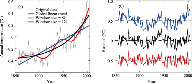
Figure 1 Adaptive algorithm used to capture the trend signals for the global annual sea surface temperature (SST): (a) original data and trends determined by global linear trend and AFA with two window sizes; (b) the residuals related to the three trends. The residuals designated as the blue and the red curves had been shifted upward and downward by 0.5, respectively.
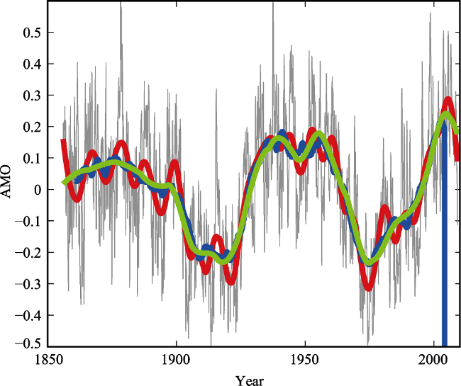
Figure 2 Adaptive algorithm used to capture the trend signals for Atlantic Multidecadal Oscillation (AMO): the detrended North Atlantic sea surface temperature anomalies data (grey) and the blue multideccadal signal are obtained from the NOAA°s website, http://www.cdc.noaa.gov/data/climateindices/List, the red and green signals are obtained by the adaptive algorithm. Clearly, the red curve is better than the blue one in tracing out the variations in the original signal, while the green curve is the best in only capturing the multidecadal oscillation.
For convenience of further analysis, we denote the original time series by x(t), and the trend signal by trend(t). Then the detrended signal is
${{x}_{detrended}}~=~x(t)-trend(t)$
To better see how this decomposition is carried out, we have shown in Figure 3 as blue and red curves the original moisture time series and the trend signals in the 4 seasons at A’rou station, where the data were measured at 4 cm below surface. As there were a lot of missing data in the measured data set, we have chosen a continuous period of the data from March 1, 2014 to February 28, 2015. This whole year long data have been partitioned into 4 lunar seasons, starting from the spring. The corresponding xdetrended signals (blue curve–red curve) are further shown in Figure 4. The small amplitude oscillations correspond to the diurnal cycle. This cycle was broken when there was rain, which was indicated by the large amplitude variations in Figures 4a-4c.
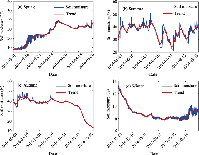
Figure 3 Adaptive algorithm used to capture the trend signals of the soil moisture at 4 cm of A’rou station in the Heihe River Basin in different seasons
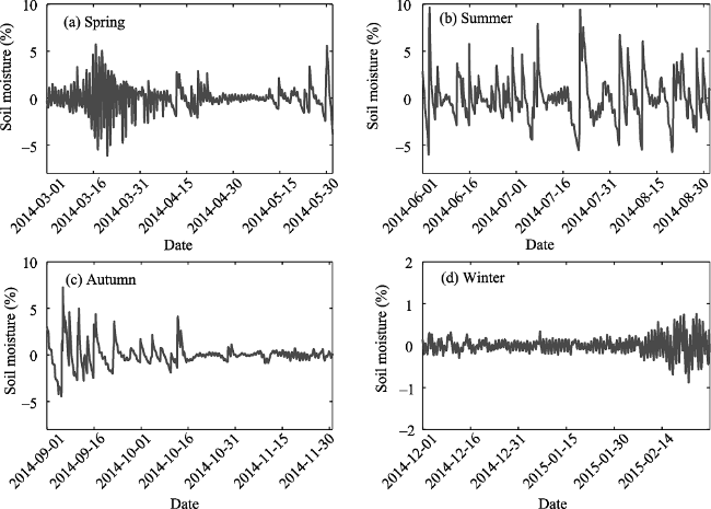
Figure 4 Adaptive algorithm used to capture the detrended data of the raw soil moisture at 4 cm of A’rou station in the Heihe River Basin in different seasons
To quantitatively assess the strength of the diurnal cycle, we can compute the power-spectral density (PSD) for the data. However, the diurnal cycle is either very weak or is totally absent if we directly use the raw data, since the trend signal there is very strong. Using the detrended signals in Figure 4, this difficulty is readily overcome. The PSD results are shown in Figures 5 for the detrended data. We observe strong spectral peaks corresponding to the diurnal cycle 1 day at two seasons, spring and winter. The first harmonic at 1/2 day can also be clearly identified. During summer, the diurnal peak at 1 day is only identifiable without the strongest signal. However, during summer, the spectral peak at 1 day is still not identifiable even when this adaptive filter is applied. The reason is that the diurnal pattern was broken or absent due to frequent rain in summer.
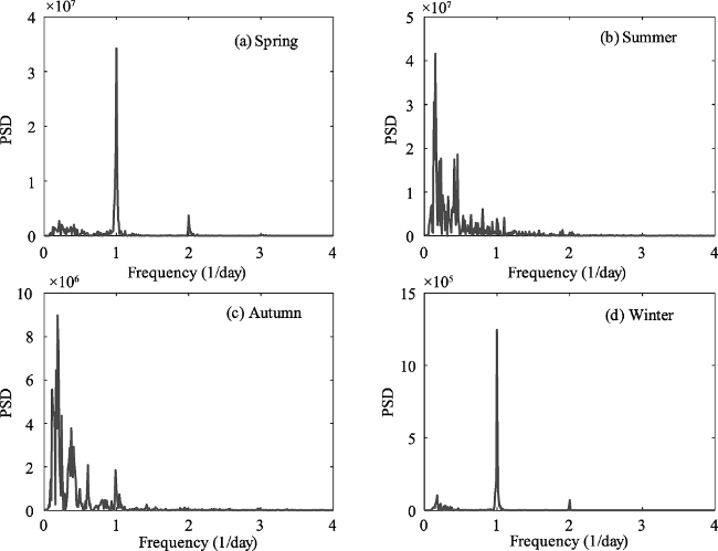
Figure 5 Power spectral density (PSD) curves for the detrended soil moisture at 4 cm of A’rou station in the Heihe River Basin in different seasons (corresponding to Figure 4)
Now that we have explained the adaptive algorithm, we can readily explain AFA. It works with a random walk process. Given a time series $\{x(1),x(2),...,\}$ with mean $\bar{x},$a random walk process y(n) is defined as
${{y}_{\left( n \right)}}=~\underset{i=1}{\overset{n}{\mathop \sum }}\,({{x}_{\left( i \right)}}-\bar{x}),\ \ n=1,\ 2,\ ...,$
Next, for a window size w, we determine for the random walk process ${{y}_{(i)}},\text{ }i=1,2,...$, a global trend ${{v}_{(i)}},\text{ }i=1,2,...$, N. Here N is the length of the random walk process. The residual, ${{y}_{(i)}}-v(i)$, characterizes fluctuations around the global trend, and its variance yields the Hurst parameter H (Gao et al., 2011b),
${{F}_{\left( W \right)}}={{\left[ \frac{1}{N}\underset{i=1}{\overset{N}{\mathop \sum }}\,{{(u\left( i \right)-v\left( i \right))}^{2}} \right]}^{1/2}}\tilde{\ }{{w}^{H}}$
To illustrate the use of AFA, we employ it to analyze how the fractal behavior of the velocity fields change with the geography of the Basin. Specifically, we consider velocity observations at the three super stations, A’rou, Daman, and Sidiaoqiao, which are at the upper, middle, and downstream area of the Basin, respectively (see Figure 6). A few examples of AFA are shown in Figure 7. We observe very good scaling behavior. However, here there are two scaling regimes, with the breaking time scale at 27$\times $10 minutes, which is about 1 day. Below this time scale, we have the shorter time scale Hurst parameter H1, which is always larger than 1, indicating nonstationarity. This means that within a day, the velocity changes a lot when the temperature changes during the diurnal cycle. On longer time scales, the Hurst parameter H2 is always larger than 1/2, but smaller than 1, indicating persistent long-range correlations. The varitions of these two Hurst parameters with the height of the measuring point are shown in Figures 8a and 8b. We observe that the variations of the Hurst parameters with height at the three stations are different: 1) the values of H1 and H2 increase from the A’rou station, which is at the upper stream of the Heihe River Basin, to the Daman station, which is at the middle stream of the Heihe River Basin, to the Sidaoqiao station, which is at the down stream of the Heihe River Basin. Overall, going from the upper to the middle and to the lower stream of the basin, the nonstationarity in the velocity field increases. This aligns well with the fact that temperature difference within a day is the largerst in the lower stream. 2) The variations of H2 with height and with stations suggest that the persistence in the correlation increases from the upper, to the middle, and finally, to the lower stream of the HRB on time scales larger than 1 day, since H2 steadily increases from the upper to the middle, and finally, to the lower stream. On the other hand, on time scales shorter than a day, whose correlation is characterized by H1, we surmise that at the upper and down stream of the Heihe River Basin, boundary layers are thin, since H1 changes with height, while at the middle stream, boundary layer is thicker and more uniform, since H1 changes little with height.
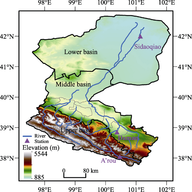
Figure 6 A schematic of the three super stations at the Heihe River Basin: A’rou station, Daman station, and Sidaoqiao station
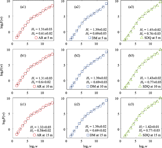
Figure 7 AFA of wind speed data at the A’rou station (a1-c1), the Daman station (a2-c2), and the Sidaoqiao station (a3-c3) at 5 m, 10 m and 15 m from January 2015 to July 2015, respectively. The slopes denoted by H1 and H2 are the Hurst parameters.

4 Multiscale analysis of geophysical data by the scale-dependent Lyapunov exponent (SDLE)

In Section 2.3, we mentioned an important issue, distinguishing chaos from noise. While many researchers are still developing new methods to tackle this problem, it is important to realize that a more fruitful direction of research is to find the defining parameters of the complex time series under study. For example, if the time series is chaotic, how do the small disturbances actually grow with time? If the time series is random, what kind of randomness is it? Cleanly answering these questions is clearly more than distinguishing chaos from noise. More importantly, under this rationale, chaos and random fractal theory are allowed to play fundamental roles simultaneously: chaos and random fractals may be relevant to the problem under study on different length scales. Underlying this rationale is the recognition of a fundamental concept, multiscale - depending upon the scale at which the signals are examined, they may exhibit different behaviors (e.g., nonlinearity, sensitive dependence on small disturbances, long memory, extreme variations, and nonstationarity), just as a great painting may exhibit various details and arouse a multitude of aesthetic feelings when appreciated at different distances, from different angles, under different illuminations, and under different moods.
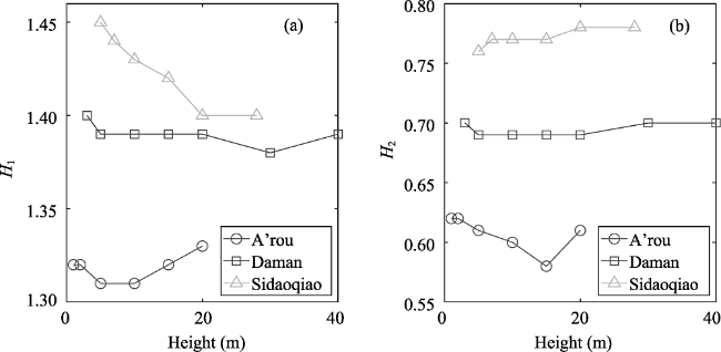
Figure 8 Variation of the Hurst parameter for wind speed with heights for the three stations: (a) short time scale H1 and (b) long time scale H2.
Hoping to characterize a complex time series on a broad range of scales simultaneously, recently, a new multiscale complexity measure, the scale-dependent Lyapunov exponent (SDLE), has been developed. SDLE was first introduced in (Gao et al., 2006c; Gao et al., 2007), and has been further developed in (Gao et al., 2009; Gao et al., 2012b) and applied to characterize EEG (Gao et al., 2011c), HRV (Hu et al., 2009a; Hu et al., 2010), financial time series (Gao et al., 2011a), and Earth's geodynamo (Ryan et al., 2008).
SDLE is a concept derived from a high-dimensional phase space. Assume that all that is known is a scalar time series$\text{ }\!\!~\!\!\text{ }x[n]=x(1),\ x(2),...,x(n)$. How can we obtain a phase space? This can be achieved by the time delay embedding technique (Packard et al., 1980; Takens et al., 1981; Saue et al., 1991). This technique is perhaps the most significant contribution of chaos theory to practical data analysis, since non-trivial dynamical systems usually involve many state variables, and therefore, have to be described by a high-dimensional state (or phase) space. The embedding technique consists of creating vectors of the form:
${{V}_{i}}=\left[ x\left( i \right),\ x\left( i+L \right),\ ...,\ x\left( i+\left( m-1 \right)L \right) \right],\ \ i=1,\ ...\text{,}\ {{N}_{p}}=n-\left( m-1 \right)L$
where the embedding dimension m and the delay time L are chosen according to certain optimization criteria (Gao et al., 2007). Specifically, L alone may be determined by computing the first zero of the autocorrelation or the first minimal point of mutual information (Fraser et al., 1986), while joint determination of m and L may be achieved using false nearest neighbor method (Liebert et al., 1991; Kennel et al., 1992) which is a static geometrical method, or time-dependent exponent method (Gao et al., 1993; Gao et al., 1994), which is a dynamical method. Note that when the time series is random, the embedding procedure transforms the self-affine (i.e. x and t have to be stretched differently in order to make the curve look “similar”, since the units for x and t are different) stochastic process into a self-similar (i.e. part of the curve in the high-dimensional space looks similar to another part or the whole when it is magnified or shrunk, since all the axes have the same unit) process in phase space. In this case, the specific value of m is not important, so long as m > 1.
After a proper phase space is re-constructed, we consider an ensemble of trajectories. We denote the initial separation between two nearby trajectories by ε0, and their average separation at time t and $t+~\Delta t$ by εt and ${{\varepsilon }_{t}}_{+\Delta ~t},$ respectively. The trajectory separation is schematically shown in Figure 9. We can then examine the relation between εt and ${{\varepsilon }_{t}}_{+\Delta ~t},$ where$\text{ }\!\!~\!\!\text{ }\Delta ~t$ is small. When $\Delta ~t\to 0,$ we have,
${{\varepsilon }_{t}}_{+~\Delta ~t}=~{{\varepsilon }_{t}}{{\text{e}}^{\lambda \left( {{\varepsilon }_{t}} \right)\Delta ~t}},$
where$\lambda ({{\varepsilon }_{t}})$ is the SDLE given by
$\lambda \left( {{\varepsilon }_{t}} \right)=~\frac{\ln {{\varepsilon }_{t+\Delta ~t}}-\ln {{\varepsilon }_{t}}}{\Delta ~t}$
Equivalently, we can express this as,
$\frac{d{{\epsilon }_{t}}}{dt}=\text{ }\!\!~\!\!\text{ }\lambda ({{\varepsilon }_{t}}){{\varepsilon }_{t}}_{t}.$
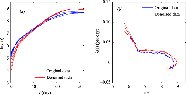
Figure 9 Detecting chaos in the Colorado River flow data: (a): error growth curves; (b): SDLE curves. The blue (solid) and red (dashed) curves are for the original and denoised data, respectively. Here, embedding parameters are m=6, L=3, and different curves are based on a few different shells described by Eq. (16). Except at the initial stage in the error growth curves, they collapse on each other.
Note that the classic algorithm of computing the Lyapunov exponent λ1 (Wolf et al., 1985) amounts to assuming ${{\epsilon }_{t}}\tilde{\ }{{\epsilon }_{0}}{{\text{e}}^{{{\lambda }_{1}}t}}$ and estimating λ1 by $(\ln {{\varepsilon }_{t}}-\ln {{\varepsilon }_{0}})/t$. Depending on ε0, this may not be the case even for truly chaotic systems, since ${{\epsilon }_{t+\delta ~t}}$ could in fact be smaller than εt. A greater difficulty with the classical assumption is that for any type of noise, ${{\lambda }_{1}}$ can always be greater than 0, leading to misclassifying noise as chaos. This is because εt will be closer to the most probable separation so long as ε0 is small (for a more quantitative discussion of this issue, see (Gao et al., 1994)). On the other hand, Eq. (13) does not involve any assumptions, except that $\Delta ~t$ is small. As we will see, chaos amounts to λ(ε) being almost constant over a range of ε.
To compute SDLE, we first determine pairs of vector$\text{ }\!\!~\!\!\text{ (}{{\text{V}}_{i}},{{\text{V}}_{j}}\text{)}$ defined by Eq. (12) which satisfy the following Inequality,
${{\varepsilon }_{k}}~\le \left| \left| {{\text{V}}_{i}}-{{\text{V}}_{j}} \right| \right|\le {{\varepsilon }_{k}}+\Delta {{\varepsilon }_{k}},\text{ }k=1,2,3,\ldots$ ,
where${{\varepsilon }_{k}}~$and$\text{ }\!\!~\!\!\text{ }\Delta {{\varepsilon }_{k}}~$are arbitrarily chosen small distances. Geometrically, Inequality (16) defines a high-dimensional shell (which reduces to a ball with radius $\Delta {{\varepsilon }_{k}}$ when ${{\varepsilon }_{k}};$ in a 2-D plane, a ball is a circle described by ${{(x-a)}^{2}}+~{{(y-b)}^{2}}={{r}^{2}}$ where (a, b) is the center of the circle, and r is the radius). We then monitor the evolution of all such vector pairs (Vi, Vj) within a shell and take the ensemble average over indices i and j. Since we are most interested in exponential or power-law functions, we assume that taking logarithm and averaging can be exchanged, then Eq. (14) can be written as
$\text{ }\!\!\lambda\!\!\text{ }\left( {{\epsilon }_{t}} \right)=\text{ }\!\!~\!\!\text{ }\left\langle \frac{~\ln \parallel {{\text{V}}_{i+t+\Delta t~}}-{{\text{V}}_{j+t+\Delta t~}}\parallel -\ln \parallel {{\text{V}}_{i+t~}}-{{\text{V}}_{j+t~}}\parallel }{\Delta t} \right\rangle$
where t and $\Delta t$ are integers in units of the sampling time, the angle brackets denote the average over indices i, j within a shell.
Readers interested in the actual code for computing SDLE are referred to (Gao et al., 2012c). Here, we summarize the distinct scaling laws of SDLE for the major models of complex data (Gao et al., 2006c):
$\bullet$ For deterministic chaos,
$\lambda (\varepsilon )\tilde{\ }\text{constant};$
$\bullet$ For noisy chaos and noise-induced chaos (Gao et al., 1999a; Gao et al., 1999b), on small scales,
$\lambda (\varepsilon )-\gamma \ln \varepsilon ,$
where $\gamma $ determines the speed of loss of information;
$\bullet$ For $1/{{f}^{2H+1}}$ processes,
$\lambda (\varepsilon )\tilde{\ }H{{\epsilon }^{-1/H}},$
$\bullet$ For $\alpha $-stable Levy processes,
$\lambda (\varepsilon )\tilde{\ }\frac{1}{\alpha }{{\varepsilon }^{-\alpha }};$
$\bullet$ For stochastic oscillations, both $\lambda (\varepsilon )\tilde{\ }-\gamma $ and $\lambda (\varepsilon )\text{ }\!\!\tilde{\ }\!\!\text{ }H{{\varepsilon }^{-1/H}}$ may be observed, depending upon which embedding parameters are used;
$\bullet$ For complex motions with multiple scaling behaviors, all the above scaling laws may be observed on different $\varepsilon $ ranges;
The last property has many interesting consequences. For example, it can readily characterize intermittent chaos, which consists of alternating regular and chaotic motions (Gao et al., 2012). In fact, this is the only method that is capable of characterizing intermittent chaos. It can also readily characterize fractal behavior mixed by periodic motions (Gao et al., 2012). Overall, with these scaling laws, clearly, distinguishing chaos from noise is no longer a problem. More importantly, these scaling laws uncover the nature of each type of models neatly. As an important application, we consider river flow dynamics, which are highly complicated, as a result of multiscale interactions between weather and climatic inputs of tremendous variability and heterogeneities in landscape properties. While efforts made in the last two decades have led to many important understandings of river flow dynamics, such as non-Gaussian (Domenico et al., 2011), heavy-tailed distributions of discharges (Anderson et al., 2011), and log-normal distributions (Bowers et al., 2012), fractal and multifractal scaling of streamflow data (Tessieret et al., 1996), increase of dimensionality (or complexity) of the flow dynamics with the scale of aggregation (Islam et al., 2002), and chaos-like behaviors (Sivakumar et al., 2004; Wang et al., 2006). A definitive answer to the nature of river flow dynamics is still lacking. Here, we ask whether the debate on whether river flow dynamics are chaotic or not can be unambiguously resolved. In researching into these issues, we have found that intermittent chaos (Pomeau et al., 1980) provides an effective framework to resolve this issue.
To understand the meaning of intermittency, let us consider the dynamics of a river flow in a certain time period (e.g., 1 year), where the time period can be partitioned into two periods, wet (e.g., rainy and snow melting) and dry. Clearly, the dynamics of the river in the wet regime will be highly complicated and different from that of the dry regime. This consideration implies that the chaotic nature of river flow dynamics cannot be detected by standard methods in chaos theory, since all classic methods for detecting chaos require the same dynamics in both wet and dry regimes.
The multiscale complexity measure SDLE is very capable of detecting intermittent chaos. One example is shown in Figure 9, for the Colorado River. Clearly, we observe exponential divergence (i.e., linear $\ln \varepsilon (t)$ vs. t for t from about 20 days to about 100-150 days). This exponential divergence gives rise to the well-defined plateaus of SDLE shown in Figure 9b (blue curves). We also note that on small scales, SDLE increases with decreasing $\epsilon $ according to Eq. (19). They correspond to the initial faster-than-exponential growth portion of the blue curves shown in Figure 9a, lasting for a time scale of less than 20 days. Such dynamics are due to stochasticity driven by snow melting, rain, etc., as well as ubiquitous measurement noise. Note that both the chaotic and the noisy dynamics shown in Figure 9 as blue curves can be improved, if we apply the adaptive algorithm discussed earlier. The results after denoising are shown as red curves in Figure 9.
Finally, we examine the physical meaning of $\text{ }\!\!\lambda\!\!\text{ (}\varepsilon \text{)}$ in the context of ensemble forecasting (Evensen, 1994; Evensen et al., 2007; Miller et al., 2007; Liu et al., 2017). First, we note that $1/\text{ }\!\!\lambda\!\!\text{ (}\varepsilon \text{)}$ is closely related to the error doubling time Tdb (Lorenz, 1995). More precisely, using Eq. (15), we have
$\ln {{\varepsilon }_{t}}=\ln {{\epsilon }_{0}}+\underset{0}{\overset{t}{\mathop \int }}\,\text{ }\!\!\lambda\!\!\text{ }\left( {{\varepsilon }_{t}} \right)\text{d}t$
The above equation readily gives the error growth curve ${{\varepsilon }_{t}},$ whose main part is given by ${{\text{e}}^{\underset{0}{\overset{t}{\mathop \int }}\,\text{ }\!\!\lambda\!\!\text{ }\left( {{\varepsilon }_{t}} \right)\text{d}t}}$. Letting ${{\varepsilon }_{t}}{{\text{T}}_{db}}=2{{\varepsilon }_{0}}$, we find the error doubling time Tdb given by
$\ln 2=\underset{0}{\overset{{{\text{T}}_{db}}}{\mathop \int }}\,\text{ }\!\!\lambda\!\!\text{ }\left( {{\varepsilon }_{t}} \right)\text{d}t$
As the first approximation, we may consider 1/$\text{ }\!\!\lambda\!\!\text{ (}\varepsilon \text{)}$ to be proportional to the doubling time. Mintz (1965) for the first time estimated the doubling time to be 5 days in the Mintz- Arakawa two-layer model. With the reduction in the initial uncertainties, it was hoped that the doubling time would increase when model complexity increases and more detailed physical processes are accounted for. However, the opposite has been observed. For example, a recent estimate of the doubling time with the ECMWF model is less than 2 days, a recent estimate of the doubling time with the ECMWF model is less than 2 days (Simmons et al., 2002). Lorenz (1995) suggests that the major factor for the decrease in the doubling time has been the increase in resolution, introducing into the system finer-scale errors that amplify more rapidly than those at the coarser scales. Although spatial resolution is not equivalent to the scale ε discussed here, they are nevertheless closely related. Therefore, the estimates of the doubling times reported so far strongly suggest that scalings described by Eqs. (19) and (20) are more relevant to reality.
SDLE analysis has been applied to analyze wind speed, air temperature, soil moisture and soil temperature measured at the HRB. Unfortunately, no chaos has been found in these variables. In future, it would be interesting to systematically explore which variables measured in the Heihe River Basin can be truly chaotic.

5 Conclusions

With the rapid accumulation of geophysical and ecological data, it has become increasingly important to find effective methods to comprehensively characterize all the available data. With this general goal and a particular goal of maximally understand the geophysical and ecological data collected in the HRB, we have advocated a complexity theory based perspective. Specifically, we have presented an adaptive multiscale filter, which can readily determine arbitrary trends, maximally reduce noise, and reliably perform fractal and multifractal analysis, and presented SDLE, which can not only reliably distinguish deterministic chaos from random processes, but also obtain the defining parameters of the process examined. We have illustrated the adaptive filter by applying it to obtain the global warming trend and the Atlantic multidecadal oscillation from sea surface temperature data, and by applying it to some variables collected at the HRB to determine diurnal cycle and fractal properties. We have also applied the SDLE to determine intermittent chaos from river flow data. Finally, SDLE has been applied to analyze wind speed, air temperature, soil moisture and soil temperature measured in the HRB. Unfortunately, no chaos has been found in these variables. In future, it would be interesting to systematically explore which variables measured in the Heihe River Basin can be truly chaotic.
[1]
Amaral L A N, Goldberger A L, Ivanov P C et al., 1998. Scale-independent measures and pathologic cardiac dynamics. Physical Review Letters, 81(1):2388-2391.

[2]
Anderson P L, Meerschaert M M , 1998. Modeling river flows with heavy tails. Water Resources Research, 34:2271-2280.

[3]
Bernaola-Galvan P, Ivanov P C, Amaral L A N et al., 2001. Scale invariance in the nonstationarity of human heart rate. Physical Review Letters, 87(16):168105.

[4]
Bowers M C, Gao J, Tung W , 2013. Long-range correlations in tree ring chronologies of the USA: Variation within and across species. Geophysical Research Letters, 40:568-572. doi: 10.1029/2012GL054011.

[5]
Bowers M C, Tung W, Gao J , 2012. On the distributions of seasonal river flows: Lognormal or power law? Water Resources Research, 48:W05536. doi: 10.1029/2011WR011308.

[6]
Box G E P, Jenkins G M , 1976. Time Series Analysis: Forecasting and Control. 2nd ed. San Francisco: Holden-Day.

[7]
Chen Y, Ding M, Kelso J , 1997. Long memory processes (1/fα Type) in human coordination. Physical Review Letters, 79(22):4501-4504.

[8]
Cheng G, Zhao W, Feng Z et al., 2014. Integrated study of the water-ecosystem-economy in the Heihe River Basin. National Science Review, 1(3):413-428.

[9]
Collins J J, Luca C J D , 1994. Random walking during quiet standing. Physical Review Letters, 73(5):764-767.

[10]
Cox D R , 1984. Long-range dependence: A review. In: David H A, David H T. Statistics: An appraisal. Ames, Iowa: The Iowa State University Press, 55-74.

[11]
De Domenico M, Latora V , 2011. Scaling and universality in river flow dynamics. Europhysics Letters, 94(5):58002. doi: 10.1209/0295-5075/94/58002.

[12]
Evensen G , 1994. Sequential data assimilation with a nonlinear quasi-geostrophic model using Monte-Carlo methods to forecast error statistics. Journal of Geophysical Research, 99(C5):10143-10162.

[13]
Evensen G , 2007. Data Assimilation, the Ensemble Kalman Filter. Berlin, Heidelberg: Springer.

[14]
Feigenbaum M J , 1983. Universal behavior in nonlinear systems. Physica D: Nonlinear Phenomena, 7:16-39.

[15]
Feng Q, Endo K, Cheng G , 2001. Towards sustainable development of the environmentally degraded arid rivers of China: A case study from Tarim River. Environmental Geology, 41:229-238.

[16]
Fraser A, Swinney H , 1986. Independent coordinates for strange attractors from mutual information. Physical Review A, 33:1134-1140.

[17]
Frisch U , 1995. Turbulence: The Legacy of A.N. Kolmogorov. New York: Cambridge University Press.

[18]
Gao J, Billock V, Merk I et al., 2006a. Inertia and memory in ambiguous visual perception. Cognitive Processing, 7:105-112.

[19]
Gao J, Cao Y, Tung W et al., 2007. Multiscale Analysis of Complex Time Series: Integration of Chaos and Random Fractal Theory, and Beyond. Hoboken, NJ: John Wiley & Sons, Inc.

[20]
Gao J, Chen C C, Hwang S K et al., 1999a. Noise-induced chaos. International Journal of Modern Physics B, 13(28):3283-3305.

[21]
Gao J, Fang P, Liu F , 2017. Empirical scaling law connecting persistence and severity of global terrorism. Physica A: Statistical Mechanics and Its Applications, 482:74-86.

[22]
Gao J, Hu J, Mao X et al., 2012a. Culturomics meets random fractal theory: Insights into long-range correlations of social and natural phenomena over the past two centuries. Journal of the Royal Society Interface, 9(73):1956-1964.

[23]
Gao J, Hu J, Mao X et al., 2012b. Detecting low-dimensional chaos by the “noise titration” technique: Possible problems and remedies. Chaos, Solitons, & Fractals, 45:213-223.

[24]
Gao J, Hu J, Tung W et al., 2006b. Assessment of long range correlation in time series: How to avoid pitfalls. Physical Review E, 73:016117. doi: 10.1103/PhysRevE.73.016117.

[25]
Gao J, Hu J, Tung W et al., 2006c. Distinguishing chaos from noise by scale-dependent Lyapunov exponent. Physical Review E, 74:066204. doi: 10.1103/PhysRevE.74.066204.

[26]
Gao J, Hu J, Tung W , 2009. Quantifying dynamical predictability: The pseudo-ensemble approach. Chinese Annals of Mathematics, Series B, 30(5):569-588.

[27]
Gao J, Hu J, Tung W et al., 2011a. Multiscale analysis of economic time series by scale-dependent Lyapunov exponent. Quantitative Finance, 13(2):265-274.

[28]
Gao J, Hu J, Tung W , 2011b. Facilitating joint chaos and fractal analysis of biosignals through nonlinear adaptive filtering. PLoS One, 6(9):e24331. doi: 10.1371/journal.pone.0024331.

[29]
Gao J, Hu J, Tung W , 2011c. Complexity measures of brain wave dynamics. Cognitive Neurodynamics, 5:171-182.

[30]
Gao J, Hu J, Tung W et al., 2012c. Multiscale analysis of physiological data by scale-dependent Lyapunov exponent. Frontiers in Fractal Physiology, 2:110. doi: 10.3389/fphys.2011.00110.

[31]
Gao J, Hwang S K, Liu J M , 1999b. When can noise induce chaos? Physical Review Letters, 82:1132-1135.

[32]
Gao J, Qi Y, Cao Y et al., 2005a. Protein coding sequence identification by simultaneously characterizing the periodic and random features of DNA sequences. Journal of biomedicine and biotechnology, 2:139-146.

[33]
Gao J, Rao N S V, Hu J et al., 2005b. Quasi-periodic route to chaos in the dynamics of Internet transport protocols. Physical Review Letters, 94:198702. doi: 10.1103/PhysRevLett.94.198702.

[34]
Gao J, Rubin I , 2001. Multifractal modeling of counting processes of long-range-dependent network traffic. Computer Communications, 24:1400-1410.

[35]
Gao J, Sultan H, Hu J et al., 2010. Denoising nonlinear time series by adaptive filtering and wavelet shrinkage: A comparison. IEEE Signal Processing Letters, 17:237-240.

[36]
Gao J, Zheng Z , 1993. Local exponential divergence plot and optimal embedding of a chaotic time series. Physical Review A, 181:153-158.

[37]
Gao J, Zheng Z , 1994. Direct dynamical test for deterministic chaos and optimal embedding of a chaotic time series. Physical Review E, 49:3807-3814.

[38]
Gilden D H, Mallon A M, Thornton M T , 1995. 1/f noise in human cognition. Science, 267(5205):1837-1839.

[39]
Hu J, Gao J, Cao Y et al., 2007. Exploiting noise in array CGH data to improve detection of DNA copy number change. Nucleic Acids Research, 35(5):e35. doi: 10.1093/nar/gkl730.

[40]
Hu J, Gao J, Tung W , 2009a. Characterizing heart rate variability by scale-dependent Lyapunov exponent. Chaos, 19:028506. doi: 10.1063/1.3152007.

[41]
Hu J, Gao J, Tung W et al., 2010. Multiscale analysis of heart rate variability: A comparison of different complexity measures. Annals of Biomedical Engineering, 38:854-864.

[42]
Hu J, Gao J, Wang X , 2009b. Multifractal analysis of sunspot time series: The effects of the 11-year cycle and Fourier truncation. Journal of Statistical Mechanics: Theory and Experiment, 2:P02066. doi: 10.1088/1742- 5468/2009/02/P02066.

[43]
Islam M N, Sivakumar B , 2002. Characterization and prediction of runoff dynamics: A nonlinear dynamical view. Advances in Water Research, 25:179-190.

[44]
Ivanov P C, Rosenblum M G, Amaral L A N et al., 1999. Multifractality in human heartbeat dynamics. Nature, 399(6735):461-465.

[45]
Ivanov P C, Rosenblum M G, Peng C K et al., 1996. Scaling behaviour of heartbeat intervals obtained by wavelet-based time-series analysis. Nature, 383(6598):323-327.

[46]
Kennel M, Brown R, Abarbanel H , 1992. Determining embedding dimension for phase-space reconstruction using a geometrical construction. Physical Review A, 45:3403-3411.

[47]
Li D, Feng J, Chen L et al., 2003. Study on interdecadal change of Heihe runoff and Qilian Mountain’s climate. Plateau Meteorology, 22(2):104-110. (in Chinese)

[48]
Li S C, Wang Y, Cai Y L , 2010. The paradigm transformation of geography from the perspective of complexity sciences. Acta Geographica Sinica, 65(12):1315-1324. (in Chinese)

[49]
Li W, Kaneko K , 1992. Long-range correlation and partial 1/ f α spectrum in a noncoding DNA sequence. Europhysics Letters, 17(7):655-660.

[50]
Li X, Cheng G, Liu S et al., 2013. Heihe Watershed Allied Telemetry Experimental Research (HiWATER): Scientific objectives and experimental design. Bulletin of the American Meteorological Society, 94(8):1145-1160.

[51]
Liebert W, Pawelzik K, Schuster H , 1991. Optimal embedding of chaotic attractors from topological considerations. Europhysics Letters, 14:521-526.

[52]
Liu F, Li X , 2017. Formulation of scale transformation in a stochastic data assimilation framework. Nonlinear Processes in Geophysics, 24(2):279-291.

[53]
Liu S M, Li X, Xu Z W et al., 2018. The Heihe integrated observatory network: A basin-scale land surface processes observatory in China. Vadose Zone Journal, 17:180072. doi: 10.2136/vzj2018.04.0072.

[54]
Liu S M, Xu Z, Wang W et al., 2011. A comparison of eddy-covariance and large aperture scintillometer measurements with respect to the energy balance closure problem. Hydrology and Earth System Sciences, 15(4):1291-1306.

[55]
Lorenz E N , 1995. Predictability: A problem partly solved. In: Proceedings of Seminar on Predictability, Reading. Berkshire, United Kingdom: European Centre for Medium-Range Weather Forecasts, 1-18.

[56]
Mandelbrot B B , 1982. The Fractal Geometry of Nature. San Francisco: Freeman.

[57]
Micklin P P , 1988. Desiccation of the Aral Sea: A water management disaster in the Soviet Union. Science, 241:1170-1176.

[58]
Miller R N , 2007. Topics in data assimilation: Stochastic processes. Physica D: Nonlinear Phenomena, 230(1):17-26.

[59]
Mintz Y , 1965. A very long-term global integration of the primitive equations of atmospheric motion: An experiment in climate simulation. In: Mitchell J M. Causes of Climatic Change. Meteorological Monographs. Boston, MA: American Meteorological Society, 22-36.

[60]
Osborne A R, Provenzale A , 1989. Finite correlation dimension for stochastic-systems with power-law spectra. Physica D: Nonlinear Phenomena, 35:357-381.

[61]
Packard N H, Crutchfield J P, Farmer J D et al., 1980. Geometry from a time series. Physical Review Letters, 45:712-716.

[62]
Peng C K, Buldyrev S V, Goldberger A L et al., 1992. Long-range correlations in nucleotide sequences. Nature, 356(6365):168-170.

[63]
Pomeau Y, Manneville P , 1980. Intermittent transition to turbulence in dissipative dynamical systems. Communications in Mathematical Physics, 74:189-197.

[64]
Provenzale A, Osborne A R, Soj R , 1991. Convergence of the K2 entropy for random noises with power law spectra. Physica D: Nonlinear Phenomena, 47:361-372.

[65]
Ruelle D, Takens F , 1971. On the nature of turbulence. Communications in Mathematical Physics, 20(3):167-192.

[66]
Ryan D A, Sarson G R , 2008. The geodynamo as a low-dimensional deterministic system at the edge of chaos. Europhysics Letters, 83:49001. doi: 10.1209/0295-5075/83/49001.

[67]
Sauer T, Yorke J A, Casdagli M , 1991. Embedology. Journal of Statistical Physics, 65(3/4):579-616.

[68]
Shen S, Ye S J, Cheng C X et al., 2018. Persistence and corresponding time scales of soil moisture dynamics during summer in the Babao River Basin, Northwest China. Journal of Geophysical Research: Atmospheres, 123:8936-8948. doi: 10.1029/2018JD028414.

[69]
Simmons A, Hollingsworth A , 2002. Some aspects of the improvement in skill of numerical weather prediction. Quarterly Journal of the Royal Meteorological Society, 128(580):647-677.

[70]
Sivakumar B , 2004. Chaos theory in geophysics: Past, present and future. Chaos, Solitons & Fractals, 19(2):441-462.

[71]
Song C Q, Cheng C X, Shi P J , 2018. Geography complexity: New connotations of geography in the new era. Acta Geographica Sinica, 73(7):1189-1198. (in Chinese)

[72]
Song C Q, Yuan L H, Yang X F et al., 2017. Ecological-hydrological processes in arid environment: Past, present and future. Journal of Geographical Sciences, 27(12):1577-1594.

[73]
Takens F , 1981. Detecting strange attractors in turbulence. In: Rand D, Young L S. Dynamical Systems and Turbulence. Lecture Notes in Mathematics. Berlin: Springer-Verlag, 366-381.

[74]
Tessier Y, Lovejoy S, Hubert P et al., 1996. Multifractal analysis and modeling of rainfall and river flows and scaling, causal transfer functions. Journal of Geophysical Research: Atmospheres, 101(D21):26427-26440.

[75]
Tung W, Gao J, Hu J et al., 2011. Detecting chaotic signals in heavy noise environments. Physical Review E, 83:046210. doi: 10.1103/PhysRevE.83.046210.

[76]
Turcotte D L , 1995. Chaos, fractals, nonlinear phenomena in earth sciences. Reviews of Geophysics, 33(Suppl.1):341-344.

[77]
Voss R F , 1992. Evolution of long-range fractal correlations and 1/f noise in DNA base sequences. Physical Review Letters, 68(25):3805-3808.

[78]
Wang P, Li Z, Gao W et al., 2011. Glacier changes in the Heihe River Basin over the past 50 years in the context of climate change. Resources Science, 33(3):399-407. (in Chinese)

[79]
Wang W, Vrijling J K, Van Gelder P H A J M et al., 2006. Testing for nonlinearity of streamflow processes at different timescales. Journal of Hydrology, 322:247-268.

[80]
Wolf A, Swift JB, Swinney H L et al., 1985. Determining Lyapunov exponents from a time series. Physica D: Nonlinear Phenomena, 6:285-317.

[81]
Wolf M , 1997. 1/f noise in the distribution of prime numbers. Physica A: Statistical Mechanics and Its Applications, 241(3/4):493-499.

[82]
Xiao S, Xiao H, Kobayashi O , 2007. Dendroclimatological investigations of sea buckthorn (Hippophae rhamnoides) and reconstruction of the equilibrium line altitude of the July First Glacier in the western Qilian Mountains, northwestern China. Tree-Ring Research, 63:15-26.

[83]
Yang J, Su K, Ye S J , 2019. Stability and long-range correlation of air temperature in the Heihe River Basin. Journal of Geographical Sciences, 29(9):1462-1474.

[84]
Zhang T, Shen S, Cheng C X et al., 2018. Long-range correlation analysis of soil temperature and moisture on A’rou hillsides, Babao River Basin. Journal of Geophysical Research: Atmospheres, 123:12606-12620. doi. org/10.1029/2018JD029094.

Outlines

/