
Journal of Geographical Sciences >
Using 137Cs and 210Pbex to investigate the soil erosion and accumulation moduli on the southern margin of the Hunshandake Sandy Land in Inner Mongolia
|
Hu Yunfeng (1974-), Associate Professor, specialized in environment monitoring & assessment and regional sustainable development. E-mail: huyf@lreis.ac.cn |
Received date: 2018-11-10
Accepted date: 2019-02-15
Online published: 2019-12-09
Supported by
Strategic Priority Research Program of CAS(No.XDA19040301)
Strategic Priority Research Program of CAS(No.XDA20010202)
National Key Research and Development Program of China(No.2016YFC0503701)
National Key Research and Development Program of China(No.2016YFB0501502)
Key Project of High-resolution Earth Observation(No.00-Y30B14-9001-14/16)
Copyright
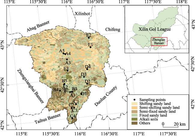
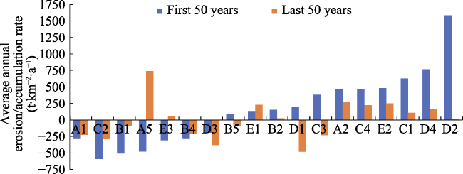
Wind-driven soil erosion results in land degradation, desertification, atmospheric dust, and sandstorms. The Hunshandake Sandy Land, an important part of the Two Barriers and Three Belts project, plays important roles in preventing desert and sandy land expansion and in maintaining local sustainability. Hence, assessing soil erosion and soil accumulation moduli and analyzing the dynamic changes are valuable. In this paper, Zhenglan Banner, located on the southern margin of the Hunshandake Sandy Land, was selected as the study area. The soil erosion and accumulation moduli were estimated using the 137Cs and 210Pbex composite tracing technique, and the dynamics of soil erosion and soil accumulation were analyzed during two periods. The results are as follows: (1) the regional 137Cs reference inventory was 2123.5±163.94 Bq/m 2, and the regional 210Pbex reference inventory was 8112±1787.62 Bq/m 2. (2) Based on the 137Cs isotope tracing analysis, the erosion moduli ranged from -483.99 to 740.31 t·km -2·a -1. Based on the 210Pbex isotope tracing analysis, the erosion moduli ranged from -441.53 to 797.98 t·km -2·a -1. (3) Compared with the earliest 50 years, the subsequent 50 years exhibited lower soil erosion moduli and accumulation moduli. Therefore, the activities of local sand dunes weakened, and the quality of the local ecological environment improved. The multi-isotope composite tracing technique combining the tracers 137Cs and 210Pbex has potential for similar soil erosion studies in arid or semiarid regions around the world.
HU Yunfeng , ZHANG Yunzhi . Using 137Cs and 210Pbex to investigate the soil erosion and accumulation moduli on the southern margin of the Hunshandake Sandy Land in Inner Mongolia[J]. Journal of Geographical Sciences, 2019 , 29(10) : 1655 -1669 . DOI: 10.1007/s11442-019-1983-1
Figure 1 The spatial distributions of plots and land in Zhenglan Banner, Xilin Gol, Inner Mongolia |
Table 1 The model estimated value, potential CRI range and measured CPIs |
| Plot | Longitude (°E) | Latitude (°N) | Elevation (m) | Annual rainfall mm·a-1 | Model estimated CRI Bq·m-2 | Potential CRI range Bq·m-2 | Measured CPI Bq·m-2 | Is the measured CPI fall within the potential CRI range? |
|---|---|---|---|---|---|---|---|---|
| A1 | 115.93 | 42.33 | 1367 | 365 | 1576 | 1890-2665 | 2864 | no |
| A3 | 115.91 | 42.74 | 1319 | 2225 | yes | |||
| A4 | 115.89 | 42.81 | 1325 | 2022 | yes | |||
| B1 | 115.9 | 42.33 | 1365 | 2455 | yes | |||
| B2 | 115.9 | 42.33 | 1366 | 1928 | yes | |||
| B3 | 115.94 | 42.33 | 1376 | 2124 | yes | |||
| B4 | 115.73 | 42.36 | 1389 | 2952 | no | |||
| B5 | 115.82 | 42.44 | 1342 | 2394 | yes | |||
| C2 | 115.9 | 42.13 | 1316 | 3256 | no | |||
| C3 | 115.94 | 42.13 | 1339 | 2904 | no | |||
| D1 | 116.09 | 42.29 | 1282 | 4635 | no | |||
| D2 | 116.21 | 42.41 | 1280 | 1987 | yes | |||
| D3 | 116.17 | 42.5 | 1426 | 3511 | no |
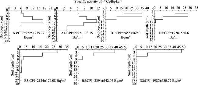
Figure 2 The 137Cs distribution patterns and CPIs in potential reference plots |
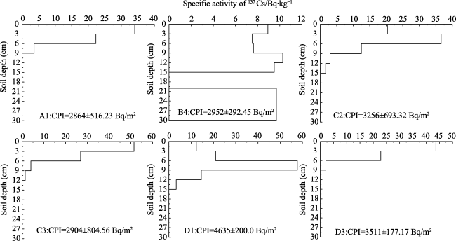
Figure 3 The 137Cs distribution patterns and CPIs in potential erosion and accumulation plots |
Table 2 137Cs activity and soil erosion/accumulation modulus estimated by the 137Cs tracing technique |
| Plot | Soil | Topography | Vegetation coverage (%) | 137Cs activity (Bq/m2) | Soil bulk density (t/m3) | Erosion /accumulation thickness (mm·a-1) | Erosion /accumulation modulus (t·km-2·a-1) |
|---|---|---|---|---|---|---|---|
| A1 | Chestnut soil | Fixed sandy land | 70-80 | 2864±516.23 | 1.56.3 | -0.144 | -224.39 |
| A2 | Chestnut soil | Semifixed sandy land (gentle slope) | 20-30 | 1332±857.16 | 1.587 | 0.170 | 269.79 |
| A5 | Aeolian sandy soil | Semifixed sandy land | 30-40 | 591±256.27 | 1.472 | 0.503 | 740.31 |
| B1 | Chestnut soil | Fixed sandy land | 70-80 | 2455±569.0 | 1.211 | -0.080 | -97.35 |
| B2 | Chestnut soil | Fixed sandy land | 70-80 | 1929±560.6 | 1.309 | 0.018 | 24.21 |
| B4 | Chernozem | Fixed sandy land | 70-80 | 2952±292.45 | 1.329 | -0.156 | -207.29 |
| B5 | Chestnut soil | Fixed sandy land | 70-80 | 2394±442.07 | 1.335 | -0.070 | -93.67 |
| C1 | Chestnut soil | Fixed sandy land | 30-40 | 1737±458.96 | 1.754 | 0.061 | 107.51 |
| C2 | Meadow soil | Fixed sandy land | 70-80 | 3256±693.32 | 1.481 | -0.196 | -290.46 |
| C3 | Chestnut soil | Fixed sandy land | 70-80 | 2904±804.56 | 1.567 | -0.149 | -233.85 |
| C4 | Chestnut soil | Fixed sandy land (hemidome) | 40-50 | 1393±97.82 | 1.473 | 0.152 | 223.44 |
| D1 | Meadow soil | Fixed sandy land | 70-80 | 4635±200.0 | 1.420 | -0.341 | -483.99 |
| D2 | Chestnut soil | Fixed sandy land | 70-80 | 1987±430.77 | 1.488 | 0.006 | 9.19 |
| D3 | Chernozem | Fixed sandy land | 70-80 | 3511±177.17 | 1.678 | -0.227 | -380.85 |
| D4 | Eolian sandy soil | Semifixed sandy land | 30-40 | 1505±254.99 | 1.363 | 0.120 | 163.44 |
| E1 | Eolian sandy soil | Fixed sandy land (piedmont platform) | 50-60 | 1451±339.53 | 1.712 | 0.135 | 231.16 |
| E2 | Eolian sandy soil | Semifixed sandy land | 30-40 | 1401±139.49 | 1.672 | 0.149 | 249.71 |
| E3 | Meadow soil | Fixed sandy land (piedmont platform) | 30-40 | 1859±222.90 | 1.632 | 0.034 | 54.81 |
Table 3 210Pbex activity and soil erosion/accumulation modulus estimated by 210Pbex tracing technique |
| Plot | Soil | Topography | Vegetation coverage (%) | 210Pbex activity (Bq/m2) | Soil bulk density (t/m3) | Erosion /accumulation thickness (mm·a-1) | Erosion /accumulation modulus (t·km-2·a-1) |
|---|---|---|---|---|---|---|---|
| A1 | Chestnut soil | Fixed sandy land | 70-80 | 9871±1298.12 | 1.56.3 | -0.164 | -255.87 |
| A2 | Chestnut soil | Semifixed sandy land (gentle slope) | 20-30 | 6483±2885.46 | 1.587 | 0.232 | 368.74 |
| A5 | Aeolian sandy soil | Semifixed sandy land | 30-40 | 7403±738.79 | 1.472 | 0.088 | 129.95 |
| B1 | Chestnut soil | Fixed sandy land | 70-80 | 11151±159.99 | 1.211 | -0.250 | -302.74 |
| B2 | Chestnut soil | Fixed sandy land | 70-80 | 7555±91.50 | 1.309 | 0.068 | 89.02 |
| B4 | Chernozem | Fixed sandy land | 70-80 | 10174±1639.76 | 1.329 | -0.186 | -247.30 |
| B5 | Chestnut soil | Fixed sandy land | 70-80 | 8118±930.08 | 1.335 | -0.001 | -0.90 |
| C1 | Chestnut soil | Fixed sandy land | 30-40 | 6609±951.43 | 1.754 | 0.210 | 368.66 |
| C2 | Meadow soil | Fixed sandy land | 70-80 | 12023±1286.46 | 1.481 | -0.298 | -441.53 |
| C3 | Chestnut soil | Fixed sandy land | 70-80 | 7713±393.57 | 1.567 | 0.048 | 74.70 |
| C4 | Chestnut soil | Fixed sandy land (hemidome) | 40-50 | 6461±1160.75 | 1.473 | 0.236 | 348.10 |
| D1 | Meadow soil | Fixed sandy land | 70-80 | 9106±147.82 | 1.420 | -0.100 | -142.62 |
| D2 | Chestnut soil | Fixed sandy land | 70-80 | 5143±662.26 | 1.488 | 0.536 | 797.98 |
| D3 | Chernozem | Fixed sandy land | 70-80 | 9966±1698.73 | 1.678 | -0.171 | -286.75 |
| D4 | Aeolian sandy soil | Semifixed sandy land | 30-40 | 5931±1660.60 | 1.363 | 0.341 | 464.27 |
| E1 | Aeolian sandy soil | Fixed sandy land (piedmont platform) | 50-60 | 7270±783.81 | 1.712 | 0.107 | 182.98 |
| E2 | Aeolian sandy soil | Semifixed sandy land | 30-40 | 6554±2132.22 | 1.672 | 0.220 | 367.25 |
| E3 | Meadow soil | Fixed sandy land (piedmont platform) | 30-40 | 8871±673.03 | 1.632 | -0.079 | -128.53 |
Figure 4 Soil erosion/accumulation modulus in two periods. A positive value indicates erosion, and a negative value indicates accumulation. |
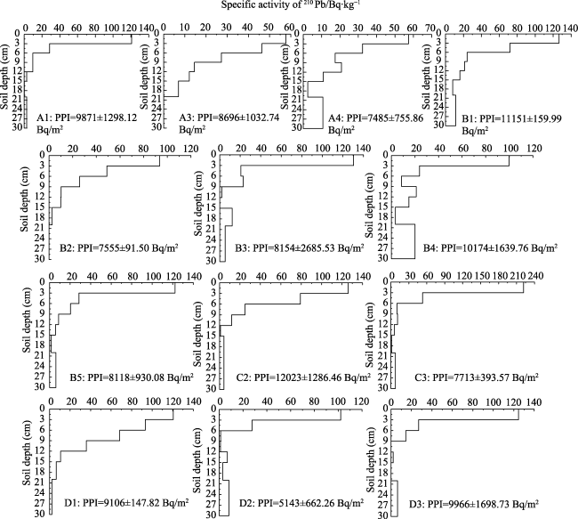
Figure 5 Vertical distributions of 210Pbex and PPIs in potential background plots |
| [1] |
|
| [2] |
|
| [3] |
|
| [4] |
|
| [5] |
|
| [6] |
|
| [7] |
|
| [8] |
|
| [9] |
|
| [10] |
|
| [11] |
|
| [12] |
|
| [13] |
|
| [14] |
|
| [15] |
|
| [16] |
|
| [17] |
|
| [18] |
|
| [19] |
|
| [20] |
|
| [21] |
|
| [22] |
|
| [23] |
|
| [24] |
|
| [25] |
|
| [26] |
|
| [27] |
|
| [28] |
|
| [29] |
|
| [30] |
|
| [31] |
|
/
| 〈 |
|
〉 |