Research Articles

Dynamics of coastline changes in Mexico

  • VALDERRAMA-LANDEROS Luis H. 1 ,
  • MARTELL-DUBOIS Raúl 1 ,
  • RESSL Rainer 1 ,
  • SILVA-CASARÍN Rodolfo 2 ,
  • CRUZ-RAMÍREZ Cesia J. 2 ,
  • MUÑOZ-PÉREZ Juan J. 3
Expand
  • 1. National Commission for the Knowledge and Use of Biodiversity, Liga Periférico-Insurgentes Sur 4903, Col. Parques del Pedregal, Del. Tlalpan, Ciudad de México. C.P. 14010, México
  • 2. Instituto de Ingeniería, UNAM, Circuito Escolar s/n, Ciudad Universitaria, Delegación Coyoacán, Ciudad de México, C.P. 04510, México
  • 3. Physical Oceanography, Cadiz University, Dpto. de Física Aplicada, CASEM 11150, Puerto Real (Cádiz), Spain

Valderrama Landeros Luis H (1974-), PhD, specialized in remote sensing. E-mail: lvalderr@conabio.gob.mx

Received date: 2017-09-26

  Accepted date: 2018-05-14

  Online published: 2019-12-09

Copyright

Copyright reserved © 2019. Office of Journal of Geographical Sciences All articles published represent the opinions of the authors, and do not reflect the official policy of the Chinese Medical Association or the Editorial Board, unless this is clearly specified.

Abstract

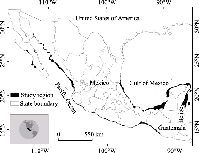
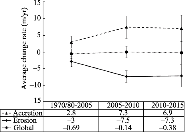
The goal of our work was to locate and quantify changes that occurred in 66% of the Mexican coastline, based on four land cover maps generated by the Mexican Mangrove Monitoring System (SMMM) of the National Commission for the Knowledge and Use of Biodiversity (CONABIO) for the years 1970/81, 2005, 2010, and 2015. Our results showed overall dominance of erosion over accretion processes, beaches being the most affected coastal land cover. Emphasis was placed on identification and description of coastline sites in which land was either continuously lost (erosion) or gained (accretion) during the studied time periods. These sites were defined as continuous unidirectional dynamic sites and were compared with previous knowledge about the geodynamics of Mexican coasts. Continuous unidirectional dynamic sites were distributed throughout the study area and within all land cover types, but predominantly corresponded to areas covered by mangroves in the states of Campeche and Nayarit. Finally, we found an intensification of coastal erosion-accretion processes over time; coastline change rates having duplicated between the earliest (1970/81-2005) and the two more recent (2005-2010, and 2010-2015) analysed time periods, with erosion rates for each corresponding period of -3 m/yr, -7.5 m/yr, and -7.3 m/yr, and accretion rates of 2.8 m/yr, 7.3 m/yr, and 6.9 m/yr, respectively.

Cite this article

VALDERRAMA-LANDEROS Luis H. , MARTELL-DUBOIS Raúl , RESSL Rainer , SILVA-CASARÍN Rodolfo , CRUZ-RAMÍREZ Cesia J. , MUÑOZ-PÉREZ Juan J. . Dynamics of coastline changes in Mexico[J]. Journal of Geographical Sciences, 2019 , 29(10) : 1637 -1654 . DOI: 10.1007/s11442-019-1679-x

1 Introduction

As zones of interface between the sea and wetlands, coastlines often have high ecosystemic value, so information about their vulnerability is important for understanding trends of change and for identifying sites having critical levels of transformation. Knowledge of local trends in coastline change due to erosion and accretion processes provides a scientific basis for developing coastal management instruments, and for the design and implementation of early warning systems to forecast and manage hydrometeorological and hydrodynamic processes, which may have effects on the population of the coast and its economic activities. Bird (1985) estimated that, worldwide, 70% of sandy beaches were undergoing erosion. In the United States, Leatherman (1988) considered coastline erosion to be critical, affecting over 90% of the country’s beaches. For the Caribbean basin, Cambers (1991), Juanes et al. (1986), and Martell et al. (2010a, 2010b) have estimated erosion rates for the beaches of the Lesser Antilles, Cuba, and Mexico.
Among the climatic phenomena generating short-term changes in coastal zones are extreme events that can cause important transformations in only a few hours (Silva et al., 2014a), such as hurricanes (Peduzzi et al., 2012), earthquakes, and tsunamis (Goff et al., 2012). The cases of the hurricanes Wilma, in 2005 (Silva et al., 2006), and Dean, in 2007 (Martell et al., 2012), both affecting the beaches around the city of Cancun, are examples of short-term impacts in Mexico. Other global climate phenomena that induce mid- and long-term changes in coastal zones are sea level rise (IPCC, 2007) and ocean acidification (Halper et al., 2008). In their research of global climate change and ocean conditions focused on wind speed and wave height, Young et al. (2011) found a general global tendency of increased wind speeds ​​and, to a lesser extent, of increased wave heights. However, in order to determine whether climatic or social factors had any effect on coastlines, Weinkle et al. (2012) performed an analysis of the points of entry of hurricanes on coastal zones. Similarly, Kunkel et al. (2012) identified a high degree of heterogeneity in the data and found no evidence of an increase in the strength of hurricanes, concluding that the intensification in damage caused to coastal zones could be the result of increased economic activity in these areas and nearby. Silva et al. (2014a) pointed out that the augmented human occupation and demographic expansion in coastal zones is one of the causes of their increased vulnerability to climatic phenomena. In a 70-year long multitemporal evaluation of the continental coast of China from 1940 to 2011, Hou et al. (2016) found the drastic anthropization of coastal zones had produced varied and complex processes of advance and retreat of the coastline, with accretion dominating (68%) over erosion (22%). Anthropogenic occupation of coastal zones possibly modifies their evolution and their capacity to recover from the effects of extreme events.
According to data from Silva et al. (2014b), about 4% of the total surface area of Mexico (1.9 million km2) is under 10 m a.s.l. in elevation in coastal zones inhabited by 10% of the total population. For these areas, sun and beach tourism is the most important economic activity in terms of employment and generation of foreign exchange revenue, receiving 60% of the total of international tourists visiting Mexico in 2012 (Diario Oficial de la Federación de México, 2013). Data from the Ministry of Tourism (SECTUR, 2015) indicate, that in 2015, a total of 32.1 million international tourists produced a revenue of US$ 17,734 million (representing 8.5% of the total GDP) and generated nearly 9 million jobs, which according to the World Tourism Organization placed Mexico ninth worldwide in attracting foreign exchange from tourism.
Since Mexico is one of the most diverse countries in the world in terms of coastal relief forms (Ortiz-Pérez and Espinosa, 1991; Sarukhán et al., 2009), Mexican coasts differ greatly in their vulnerability to erosive and accumulative processes (Inman and Nordstrom, 1971). At one extreme, erosive coastal processes and sea level changes have formed cliffs and coastal terraces over a long period of time. At the other extreme, the shallow, accumulative coastal regions in wetlands, mangroves, and beaches are susceptible to modifications over very short time periods, mainly due to atmospheric and marine forces (Shepard, 1963). While previous studies by Martell et al. (2010a; 2010b; 2012), Escudero et al. (2014), Odéris et al. (2014), Martínez et al. (2014), and Delgadillo-Calzadilla et al. (2014) analysed the evolution of the Mexican coastline and identified erosive processes on specific coastal stretches, to date no quantitative nationwide study of Mexico has been made. The purpose of this work, therefore, was to identify and quantify both the magnitude and the tendencies of the erosion and accretion processes that have taken place in 66% of the Mexican coastline between 1970 and 2015.

2 Materials and methods

2.1 Study area

The study area was delimited by the cartography derived by the Mexican Mangrove Monitoring System (SMMM) of the National Commission for the Knowledge and Use of Biodiversity (CONABIO). The mangrove areas studied, and the surrounding zones as defined by CONABIO, were based on several criteria, the most relevant including: mangrove patches larger than 1 ha identified in satellite imagery (SPOT-5) of 2005, 2010, and 2015; a 5-km buffer around these patches (2005); polygons of Natural Protected Areas defined by the National Commission of Natural Protected Areas (CONANP, 2008); and Ramsar sites (Rodríguez-Zúñiga et al., 2012). The study area is distributed over all 17 coastal states of Mexico, with mangrove coverage along the eastern (Atlantic) and western (Pacific) coasts (Figure 1) covering an area of 86,241 km2 (representing 66% of the country’s total coastline of 11,592 km) (SAGARPA, 2015). Despite focusing on mangrove land cover, the study area comprises nearly all types of the Mexican coast, excluding only the Northeastern Gulf of Mexican Coast, the Northwestern Pacific Coast, and the Upper Gulf of California Coast. The characteristics and extension of the study area are further discussed in Section 2.4.
Figure 1 Study area: National Mexican coastline with mangrove coverage derived by the SMMM of CONABIO (2005)

2.2 SMMM cartography and coastlines

The mangrove distribution maps were produced by CONABIO (http://geoportal.conabio. gob.mx/) using satellite imagery (basically SPOT-5 satellite images) and aerial photographs for four dates: 1970/81 (not all of the coastline could be covered with data from 1970), 2005, 2010, and 2015. The methodology applied is described in Valderrama et al. (2014) and Rodríguez-Zúñiga et al. (2012). Table 1 shows the classification scheme in nine land cover/land use classes. Areas covered by clouds and cloud shadows were classified as Others. The maps in Lambert Conformal Conic projection were published in digital formats with a minimum cartographic area of 1 ha. With the objective of documenting the changes occurring along the coastline and the distribution of mangroves, the buffer used for defining the study area extended 5 km both inland and towards the ocean.
Table 1 Land cover/land use classification scheme applied in the SMMM
Class Description
Anthropogenic development Urbanisation, aquaculture and salt ponds, shrimp farms, roads and highways, and hydraulic infrastructure including canals
Livestock farming Land used for temporary agriculture, irrigation, livestock pastures, production of food, perennial woody monocultures typical of each region, other agroecosystems, and fallow lands
Other vegetation Shrubland and arboreal vegetation of evergreen low forests, floodable subdeciduous forests, and different types of secondary arboreal, shrubby, and herbaceous vegetation
Without vegetation Areas with no apparent vegetation, coastal sand dunes, and beaches
Mangrove Shrubby and arboreal wetlands with one or more species of mangrove: white mangrove (Laguncularia racemosa), red mangrove (Rhizophora mangle), black mangrove (Avicennia germinans), and buttoned mangrove (Conocarpus erectus)
Disturbed mangrove Wetlands made up of patches of trees and dead or regenerating mangrove shrubs. This category refers to forest cover disturbed by hurricanes, storms, and cyclones, as well as wetlands disturbed by building
Other wetlands Popal-tular-carrizal hydrophilic vegetation, floodable grasslands, hydrophilic or halophytic vegetation with individual dispersed mangroves, or small islets and coastal salt marshes with scarce vegetation cover
Water bodies Ocean, bays, estuaries, lagoons, rivers, dams, sinkholes, and shallow sinkholes
Others Cloud cover and cloud shadows
The coastline for each observation period was defined by digitizing the waterline from the satellite images, deriving the boundary between the ocean and the terrestrial coverage. Thus, for each map it was possible to define a momentaneous coastline position (Boak and Turner, 2005) and to compare the changes that occurred over 45 years (1970/80-2015). The momentary waterline only gives an approximation of the real coastline’s position, as the shoreline is determined by various local parameters, e.g., the effect of tides. Because satellite images and aerial photographs were not available for the same day(s) of each year, even less so for the same hour of the day, the analysis did not consider factors such as barometric pressure, tidal and wave effects, and daily or seasonal fluctuations. This was especially true for the aerial photographs of 1970 to 1981. According to data of the mean maximum levels of high tide, medium tide, and low tide from the Mexican Ministry of the Navy (SEMAR), the strongest tidal effects occur in few places in the north of Mexico outside the study area, (SEMAR, 2018). However, uncertainty was considered, to account for the spatial resolution of the SPOT images used for the elaboration of the maps for the years 2005, 2010, and 2015. This uncertainty depends on the resolution of the SPOT images (10 m) and the numbers of pixels needed to distinguish a spatial characteristic, which according to Rodríguez-Zúñiga et al. (2012) is of at least three pixels. Another source of error can be attributed to the georeferencing process of the images, which is related to the number of pixels needed to identify a feature in the image in order to define the control points. For these two latter sources, a total maximum possible error value can be estimated as follows:
Emp = (Ere2 + Egr2)1/2
where Emp is the maximum possible error, Ere2 is the error due to the resolution of the inputs, and Egr2 is the product error of the image georeferencing process. The estimated Emp for these sources would then be 42.4 m, which is inappropriate for accurate site-level studies, but is sufficient for national studies considering long-term trends.
In this study, the coastline change analyses were performed in segments by pairs of dates, documenting changes for the periods 1970/81-2005, 2005-2010, and 2010-2015.

2.3 Transect analysis using the Digital Shoreline Analysis System (DSAS)

The Digital Shoreline Analysis System (DSAS) is an application developed by the United States Geological Service (USGS) that works within ArcGis (V.10x). The first versions of DSAS were programmed in C for ArcInfo systems. Version 2.0 was developed in Avenue for ArcView 3.x, DSAS 3.0 for ArcGIS 9x, and the final version 4.3.4730 for ArcGIS 10x (Thieler et al., 2009).
DSAS estimates change statistics for coastline transects at different observation times. These transects are perpendicular lines drawn equidistantly from their origin on a baseline. The program generates the perpendiculars, which must be long enough to cross the coastlines analysed.
The baselines from which the perpendiculars were generated were generally drawn parallel to the most recent coastline. Depending on the coastal morphology, some baseline sections were drawn parallel to previous coastlines. The coastline positions are representative of the respective year, as were the lines. In the case of the coastline segments obtained from the 1970/81 map, the year of each line segment was based on the metadata of the aerial photographs, taking into account the wide range of dates of the photographs used. In total, 56,298 equidistant transects were generated on the baseline every 100 m along the length of the coastline of the SMMM maps; in order to include small mangrove patches, the minimum mapping unit was 1 ha.
The main indicators thus obtained are the net shoreline movement, which is the distance in meters between the intersecting lines (transect-coastline) (Figure 2) and the end point rate (m/yr), which corresponds to the net displacement of the analysed coastlines observed over the years.
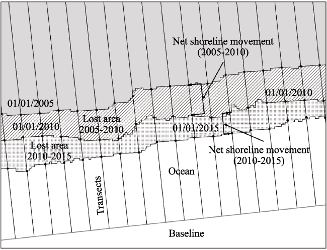
Figure 2 Illustration of example for shoreline displacement analysis for observed time periods

2.4 Land cover changes and identification of sites with recurring changes in the same direction in different periods

Using the land cover change information from the SMMM maps, the area of land affected (either by accretion or by erosion) was estimated for each coastline segment and the type of land cover was accordingly identified (Table 1). The resulting land cover polygons between each pair of lines show the type of land cover before and after the erosion/accretion process. Where the coastline displacement showed a significant trend towards erosion or accretion, the occurrence of changes in either direction over time was identified, and coastline sections in which land was either lost (erosion) or gained (accretion) were labelled as continuous unidirectional dynamic sites.
Sites displaying a continuous dynamic towards erosion or towards accretion were visualized by polygons showing land cover change and were superimposed on the SMMM land cover change maps in order to determine associations between the processes of coastline change and the physiographic conditions of the coast. The results were analysed using the Mexican Coast Classification System proposed by Silva et al. (2014b), developed at a 1:2,000,000 scale. This classification system ranks coastal zone characteristics: climatic regions, hydrographical basins, topography, and geomorphology, also taking into consideration the hydrodynamic processes and threats affecting the coast. It divides the Mexican coasts into 14 regions, in agreement with the studies of Ortiz-Pérez and Lanza-Espino (2006): nine in the Pacific and five in the Atlantic watersheds. Figure 3 presents the distribution of the regions or coastal units identified by Silva et al. (2014b) and by Ortiz-Pérez and Lanza-Espino (2006), and Table 2 summarizes their characteristics.
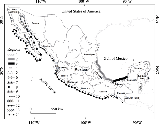
Figure 3 Coastal dynamics regionalization in the Mexican coastline according to Silva et al. (2014b). Numbers 1 to 14 correspond to the identification code assigned for each region.
Table 2 Characteristics of the 14 Mexican coastal units and regions
Coastal unit Region Description Coastal
length (km)
Gulf Zone. Includes the entire Gulf of Mexico basin. The El Lazo warm current influences the region. The unit includes four regions:
1 Northeastern Gulf of Mexican Coast Climate: temperate humid with summer rain (Cw; García, 1988).
Average annual precipitation: around 800 mm.
Sediments: fine sand - according to the classification of Wentworth (1922).
Contribution of fluvial sediments: deltaic system of the Rio Bravo. Accumulative low elevation sandy beach coasts.
558
2 Central Eastern Gulf of Mexican Coast Climate: warm subhumid with summer rain (Aw; García, 1988).
Sediment transport: dominantly from north to south.
The coast is accumulative and mixed (accumulative-erosive). Low beaches and coastal dunes are prevalent in some zones.
896
3 Central Southern Gulf of Mexican Coast Climate: warm humid with summer rains (Am; García, 1988).
Sediments: very fine clay (Wentworth, 1922).
The Tabasco deltaic complex contains very thick sediments with subsidence of the terrain structure.
596
4 and 5 Yucatan Peninsula and Caribbean Sea Coast Climate: warm subhumid with summer rain (Aw; García, 1988).
Subjected to tropical cyclones and Nortes (anticyclone cold front systems or Central American Cold Surges). The terrain drains through an underground drainage network.
Sediment transport: dominantly towards the west.
The Caribbean presents a narrow coral reef barrier parallel to the coastline. Lithified or consolidated beach strings covered by loose sand.
Sources of sediment: from Central American coasts.
1226
Coastal unit Region Description Coastal
length (km)
Baja California Peninsula Western Coast Unit. The zone receives influence from the cold Californian current descending from the north and has numerous bays. Subdivided into two regions:
6 Northwestern Pacific Coast Climate: semidry with winter rain (Bs; García, 1988)
Low precipitation and weak runoff. The coast is exposed to constant and intense distant waves.
Dominant sediment transport: southbound direction.
786
7 Southwestern California Peninsula Coast Climate: very arid with winter rains (Bw; García, 1988).
Much of the coast is subject to terrain sinking due to tectonic tilt.
1326
Gulf of California Unit. Semi-enclosed body of water influenced by circulation and tidal effects with a pronounced bathymetric gradient. Subdivided into three regions:
8 Eastern Baja California Peninsula Coast Climate: very arid with summer rain (Bw; García, 1988).
Precipitation: less than 400 mm annually.
Presents small pocket bays or inlets.
989
9 Upper Gulf of California Coast Climate: very arid with summer rain (Bw; García, 1988).
Precipitation: less than 300 mm a year.
The mouth of the Colorado River exerts an important geomorphological influence.
1164
10 Eastern Lower Gulf of California Coast Climate: semidry with winter rain (Bs; García, 1988).
This region has an important presence of coastal lagoon environments, water sources, and delta systems that dominate the sedimentary environments.
1043

Tropical Mexican Pacific Unit. Presents a significant number of coastal lagoons, lagoon-estuarine systems, bays, bars, and sandy beaches. Subdivided into four regions:
11 Western Mexican Pacific Coast Climate: warm subhumid with summer rain (Aw; García, 1988).
Annual precipitation: from 800 mm (northern sector) to a little over 1500 mm (southern sector).
Subject to the surge of tropical storms and hurricanes. Presents marshes, flood plains, and coastal lagoons.
617
12 Southwestern Mexican Pacific Coast Climate: warm subhumid with summer rain (Aw; García, 1988).
Distribution of rainfall: ranging from 400 (northern sector) to 1000 mm (southern sector).
Presents subduction. The dominant swell is of the distant type.
1433
13 Gulf of Tehuantepec Coast Climate: warm subhumid with summer rain (Aw; García, 1988).
Geologically, corresponding to a coast formed by the collision between the oceanic Cocos Plate and the continental American Plate.
508
14 Southern Mexican Pacific Coast Climate: warm subhumid with summer rain (Aw; García, 1988).
Sandy, thick and medium texture, steep slope beaches.
Sediment transport: dominantly in the SSE direction towards the Gulf of Tehuantepec. The dominant wave type is distant high energy coming from the south.
210
The sites with recurrent unidirectional changes were also compared with the map of geodynamic processes of Silva et al. (2014b), which describes the change trends of the coastline defined as a function of its tectonic characteristics, morphological expressions (erosion and accumulation forms), and hydrological and hydrographical characteristics of the estuarine and fluvial networks (Figure 4). This classification is an extension of the previous study of Ortíz Pérez and Méndez Linares (2004), who used multitemporal data from satellite images, aerial photographs, and field verification.
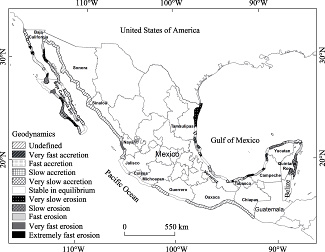
Figure 4 Coastal geodynamic classification according to Silva et al. (2014b)

3 Results and discussion

3.1 Identification of changes with DSAS

The change dynamics differ noticeably between the periods 1970/81-2005, 2005-2010 and 2010-2015. The longest time interval (1970/81-2005) showed the highest dynamic in changes (some type of coastline change was identified in 41% of the transects), a result that was expected, due to the long time lapse (24-35 years) (Figure 5). The 2005-2010 period presented less change, with only 12% of transects showing some kind of coastline alteration. In the most recent period (2010-2015), the coastline change dynamics intensified significantly, with 36% of all transects showing changes over this 5-year time interval.
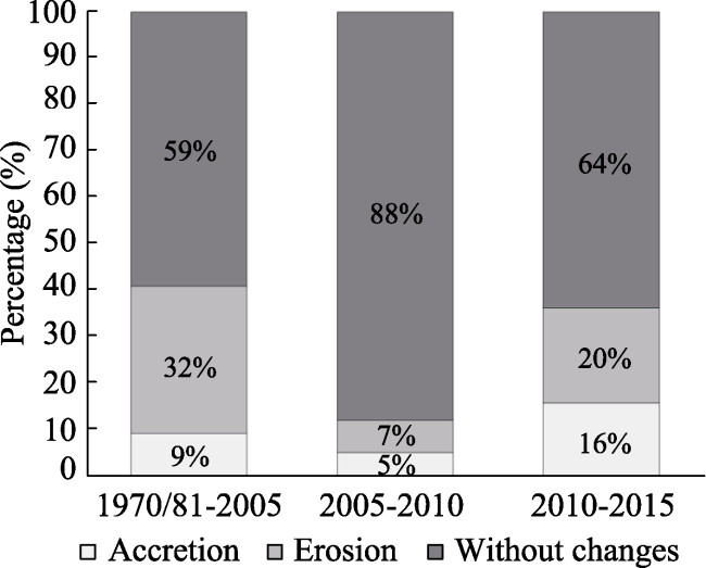
Figure 5 Percentages of national coastline change dynamics identified from transects for the three time periods studied (1970/81-2005, 2005-2010, and 2010-2015)
Figure 6 illustrates the proportion of displacements measured on the coastline in each of the three periods, both towards the land (erosion, expressed in negative numbers) and towards the ocean (accretion, expressed in positive numbers). The earliest and longest period (1970/81-2005) showed more intense coastline change dynamics; with displacements towards the land (erosion) averaging -86 m, with half of the data (first and third quartiles) in the range of -30 m and -53 m. The movements towards the ocean (accretion) showed an average of 78 m, with a distribution (first and third quartiles) between 36 m and 17 m. Both types of displacement showed significant atypical data, corresponding to extreme changes in various regions of the country. These extreme values stretched from -871 m towards the land in Laguna de Altata, Sinaloa, to 755 m towards the ocean in Laguna de Mar Muerto, Chiapas. Figure 6 also illustrates that, in the case of erosion, the most recent period (2010-2015) had some extreme values that reached a maximum of -1143 m, while in the previous period (2005-2010) the maximum erosion value only reached -248 m; these extreme data increased the value of the mean erosion. Differences in accretion records were also reflected in the extreme values, although they were less pronounced than those from the cases of erosion, reaching absolute values of only 530 m (2005-2010) and 412 m (2010-2015).
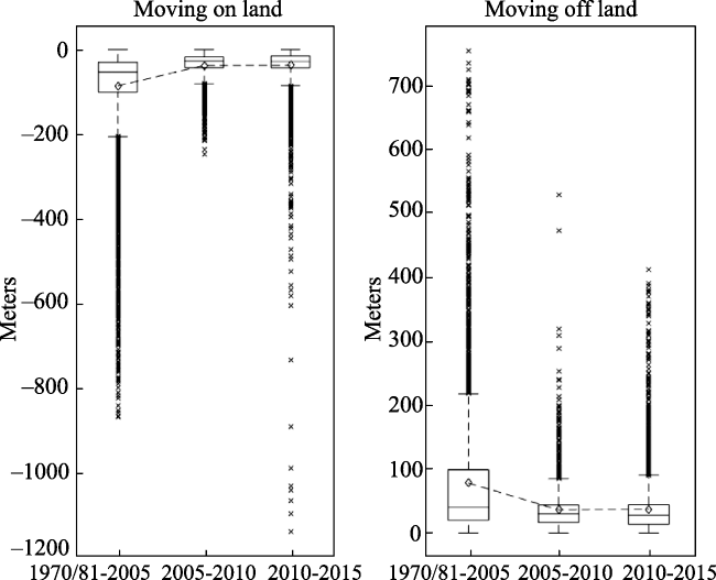
Figure 6 Distribution of net coastline displacement observed in the study area for the three time periods studied (1970/81-2005, 2005-2010, and 2010-2015). The box represents the range of values of one half of the total data from transects. The horizontal line inside the box represents the median. The rhombus indicates the mean. The vertical lines extending from the box (whiskers) represent the data having values outside 50% of the data, but within 1.5 times the height of the box or interquartile range. Atypical data are plotted outside the box.
The second and third observation periods (2005-2010 and 2010-2015) showed fewer changes with respect to the first time interval (Figure 6 and Table 3), as was expected for these shorter time periods (5 years). The mean erosion for the 2005-2010 and 2010-2015 periods was practically the same (-37 m), differing by only half a meter between both periods, and its distribution was almost identical between the first and third quartiles. A similar dynamic was observed for the accretion processes. The differences between the two periods were considered to be due to atypical causes.
Table 3 Changes in erosion and accretion statistics in the study area
Statistics Erosion (m) Coastal accretion (m)
1970/81-2005 2005-2010 2010-2015 1970/81-2005 2005-2010 2010-2015
Maximum -871 -248 -1143 755 530 412
Average -86 -37 -37 78 36 37
First quartile -30 -17 -15 20 17 13
Third quartile -101 -43 -43 99 44 44
All identified maximums were located at river mouths or in the mouths of bars and barrier islands. The erosion and accretion maximums observed in the 1970/81-2005 period and the erosion maximums in the 2005-2010 period were very similar, both being localized in the Bocana Sur barrier island of Bahía Magdalena (25.277415°, -112.133247°) in the state of Baja California Sur (Figure 7). The erosion maximum for the 2010-2015 period was the highest of all (-1143 m), and was observed at Laguna de Altata, Sinaloa (24.521790°, -107.824511°). The accretion maximum (530 m) for the 2005-2010 period was documented in Laguna de Mar Muerto, Chiapas (15.982907°, -93.951031°), and for the 2010-2015 period, the maximum accretion (412 m) was recorded in Holbox, Quintana Roo (21.543336°, -87.353128°). These sites are located in zones where the ocean interacts with lagoon systems and where the sediment transport is more dynamic than in other types of coasts, and thus, the space between barrier islands and river mouths is more susceptible to extraordinary accretion and erosion events.
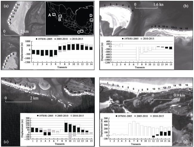
Figure 7 Sites with maximum erosion and accretion rates. a) Isla Magdalena, Baja California Sur; b) Laguna de Altata, Sinaloa; c) Laguna de Mar Muerto, Chiapas; and d) Isla de Holbox, Quintana Roo. Photographs correspond to the panchromatic band of Landsat 8 (15 m resolution), images taken on 13/08/2015, 23/10/2016, 15/01/2016, and 30/09/2015, respectively.
In detailed transect analysis the recorded changes were more dramatic and showed an increase in coastline change dynamics, with erosion processes being more prevalent than accretion processes. It would be expected that the absolute extreme values were found in the longest period, as there would be more time to accumulate changes, however, this only happened in the cases of accretion (Table 3). For the erosion phenomena, the absolute maximum corresponded to the most recent time period, of only 5 years.
The average end point rate estimated by the transects for the entire study area (Figure 8) was -0.69 m/yr for the first time period (2.8 m/yr for changes due to accretion and -3.0 m/yr for changes due to erosion), -0.14 m/yr for the second time period (7.3 m/yr for accretion and -7.5 m/yr for erosion), and -0.38 m/yr for the most recent time period (6.9 m/yr for accretion and -7.3 m/yr for erosion). This suggests that the severity and dynamic of these phenomena have increased in the last two decades. According to Landsea et al. (1999) and Goldenberg et al. (2001), this increased severity of accretion and erosion of coastlines is probably due to a natural increase in the frequency of extreme hydrometeorological phenomena. But it also may be due to the negative synergies of human activities and infrastructure developments on the coast, which cause modifications to sediment flows either directly on the coast or in the area of influence of the watershed (Silva et al., 2014a). Finally, it was observed that erosion processes were more common than accretion processes, mostly occurring during the 2005-2010 time period (-7.5 m/yr).
Figure 8 Average overall coastline change rates in the study zone by type (accretion or erosion) and time period. Bars represent half of the standard deviation.

3.2 Types of land cover affected by coastline changes

Figure 9 shows the type of land cover affected by the coastline changes. During the three periods, the land cover class Without vegetation, which mainly corresponds to beaches, was affected most commonly. Accretion processes in areas classified as Without vegetation were recorded on 82.6% (9913 ha) of the total gained land surface. Erosion processes in the Without vegetation land cover class caused 73% (-18,123 ha) of the total area of land lost (Table 4). Transect analysis showed that in the earliest time period (1970/81-2005) a significant percentage of overall coastline change took place, accretion being the cause in 51.5% of the coastline, and erosion in 71.2% of the coastline (Figure 5). In the most recent period (2010-2015) a net increase in coastline change dynamics was observed, representing up to 32.5% of the total changes produced by accretion processes and 18% of the total area involved in erosion during the three observation time periods. In total, between 1970/81 and 2015, 12,003 ha were affected by accretion and 24,811 ha were eroded.
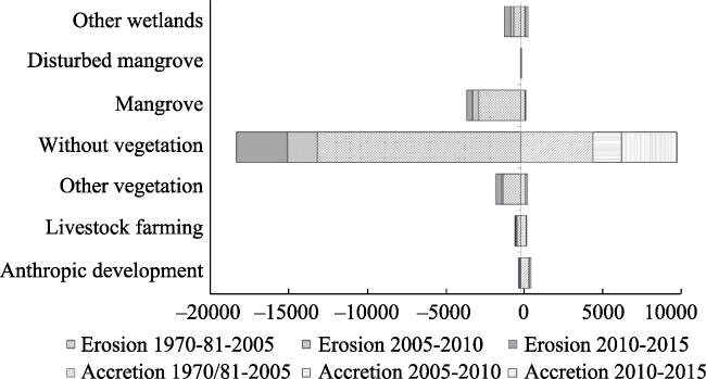
Figure 9 Erosion and accretion by period and land cover class
Table 4 Percentage of land cover type affected by accretion and erosion for each time period
Type Accretion (%) Erosion (%)
1970/81-
2005
2005-
2010
2010-
2015
Total 1970/81-
2015
1970/81-
2005
2005-
2010
2010-
2015
Total 1970/81-
2015
Anthropogenic development 4.1 0.1 0.9 5.1 0.3 0.1 0.3 0.7
Livestock farming 2.6 0.1 0.1 2.8 1.1 0.2 0.2 1.6
Other vegetation 2.4 0.1 1.0 3.4 4.7 0.4 1.3 6.4
Without vegetation 38.1 15.2 29.3 82.6 52.3 7.7 13.1 73.0
Mangrove 2.2 0.0 0.2 2.4 10.9 1.5 1.4 13.9
Disturbed mangrove 0.0 0.0 0.0 0.0 0.0 0.0 0.0 0.0
Other wetlands 2.0 0.5 1.1 3.6 1.9 0.8 1.6 4.3
Total per period 51.5 16.0 32.5 100 71.2 10.8 18.0 100
Within the accretion processes, the remaining classes of land cover represented only 17.4% of the cumulative total for the three time periods. In descending order, these land covers were: Anthropogenic development (5.1%), Other wetlands (3.6%), Other vegetation (3.4%), Livestock farming (2.8%), and Mangrove (2.4%). This shows that 5.1% of the areas gained from the oceans were caused by, or corresponded to, some kind of coastal infrastructure. In the case of erosion processes, the land cover class Mangrove (cumulative total 14% for the three periods) was the most affected after Without vegetation, followed by Other vegetation (6.4%), Other wetlands (4.3%), Livestock farming (1.6%), and Anthropogenic development (0.7%).

3.3 Identification of sites with a continuous unidirectional trend

The observation intervals for the coastline change analysis were not short enough to determine whether the changes identified occurred in a few events, such as hurricanes or river floods, or whether they were the result of less dramatic, constant accumulation or erosion processes. According to Boak and Turner (2005), obtaining the position of the coastlines as we did in this study does not allow for establishing normal or average conditions. However, the procedure we applied allowed to determine the areas with coastline changes and to identify, for the 45 years analysed, sites with constant erosion or accretion processes. The trigger factors for these unidirectional trends might be global phenomena, such as climate change, or local causes, such as the development of infrastructure modifying the local dynamics of currents and sediment supply. As shown in Figure 10, sites with continuous unidirectional coastline change are not concentrated in a single region, but are distributed along the entire littoral zone, except for the states of Tamaulipas and Veracruz on the Gulf of Mexico, and Michoacán and Baja California on the Pacific.
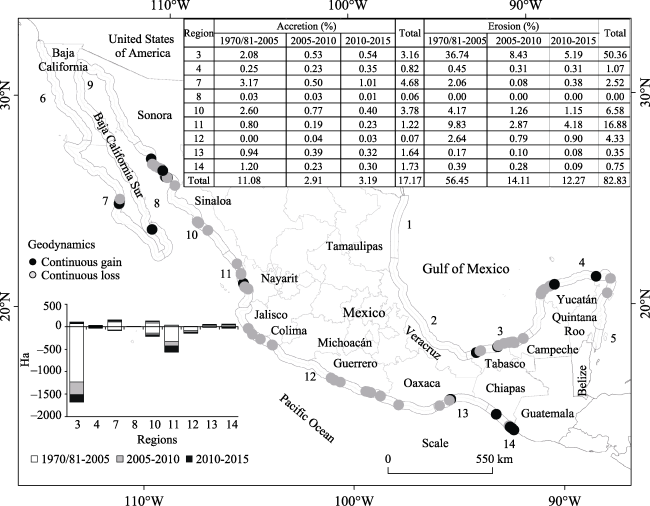
Figure 10 Sites showing continuous unidirectional coastline change (erosion or accretion over all three observation periods) with area in hectares, and accretion/erosion percentages for each period
The total area affected by processes showing continuous unidirectional coastline change dynamics between 1970/81 and 2015 was 3334 ha. Considering the typological classification of the coastal zone of Mexico proposed by Silva et al. (2014b), the coastal units designated as Region 3 (Central Southern Gulf of Mexican Coast) and Region 11 (Western Mexican Pacific Coast) comprised 72% of the total area affected by continuous coastline change dynamics (Figure 10). Deposition processes characterize Region 3, predominated by accumulation of delta sediments, conditions that are optimal for ecosystems such as mangroves. This is one of the reasons why the states of Tabasco and Campeche together account for one-third of the total mangrove area in Mexico (Rodríguez-Zúñiga et al., 2012). However, mangroves are one of the most sensitive ecosystems if the sedimentation regime is modified (Lovelock et al., 2007) and are most at risk under rising sea level scenarios (Hernández- Santana et al., 2008). As above-mentioned, from 1970/81 to 2015 the erosion processes in Region 3 represented 50% of the total area affected by a continuous unidirectional change. In that same period, accretion processes represented 3% of the total surface affected by some form of continuous unidirectional change.
Region 11, also characterized by swamps and flood plains, contains 18% of the surface affected by continuous unidirectional changes. Region 7 (Southwestern California Peninsula Coast), corresponding to the Pacific slope of the Baja California Peninsula, had the highest percentage of accretion processes (5% of the total region’s surface). All other regions together only accumulated 11% of the surface affected by continuous unidirectional coastline change processes, most of which were of erosion.
Table 5 shows the number of transects, the average distance (length) of change, and the maximum and minimum values during the study period per state, indicating the type of coastline change (accretion or erosion). The average displacement found for all the coastlines (280 m due to accretion and -398 m due to erosion) illustrates that erosion processes are more prevalent than accretion processes. In the states of Campeche, Colima, Guerrero, Jalisco, and Sinaloa no continuous processes of accretion (Figure 10) were recorded. Campeche showed the largest number of cases of erosion and the highest average length of displacement.
Table 5 Number of transects representing processes of continuous unidirectional coastline change with average, maximum, and minimum length of coastline change per state
State Accretion Erosion
Transects Average length 1970/81-
2015 (m)
Maximum length 1970/81-
2015 (m)
Minimum length 1970/81-
2015 (m)
Transects Average length 1970/81-2015 (m) Maximum length 1970/81-
2015 (m)
Minimum length 1970/81-2015 (m)
Baja California Sur 33 518.8 807.7 130.3 5 -389.9 -456.2 -151.3
Campeche 225 -683.0 -1012.9 -72.9
Chiapas 14 349.9 688.9 56.7 5 -243.2 -256.0 -231.9
Colima 28 -112.5 -149.9 -66.2
Guerrero 37 -110.7 -178.3 -31.5
Jalisco 10 -130.4 -202.3 -37.8
Nayarit 18 175.2 332.0 77.9 147 -412.2 -1027.0 -40.4
Oaxaca 24 192.0 270.7 114.6 11 -182.4 -232.3 -93.3
Quintana Roo 1 69.8 69.8 69.8 4 -78.1 -108.9 -42.9
Sinaloa 5 -214.0 -519.0 -16.8
Sonora 29 293.8 432.2 39.9 102 -158.7 -344.0 -36.2
Tabasco 47 201.9 246.3 73.9 22 -361.5 -548.5 -74.3
Yucatan 9 133.7 201.1 50.3 42 -63.7 -110.2 -34.9
Total 175 280.4 807.7 39.9 643 -398.4 -1027 -16.8
Figure 11 shows the accumulated area for land cover classes affected by coastline change dynamics in sites identified with unidirectional changes per state for the three time periods. The areas affected by erosion processes (2761 ha) are almost 5 times higher than those affected by accretion (572 ha), due mainly to the number of cases recorded in Campeche and Nayarit, where the main land cover type affected was Mangrove. For accretion cases, the areas are mainly in the Without vegetation land cover class, except in the state of Tabasco, where most of this area was occupied for agricultural and livestock activities.
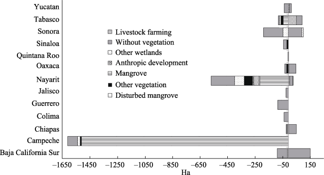
Figure 11 Land cover classes in sites identified as of continuous unidirectional accretion or erosion by coastal state
The geodynamic analysis elaborated by Silva et al. (2014b) indicates the expected dynamics of change on the Mexican coastline. Complete concordance with Silva et al. (2014b) was found in the case of Tabasco and Campeche (Region 3), where the geodynamic map shows an extremely rapid coastline regression. This dramatic dynamic is confirmed through 171 transects measuring average losses of -597 m between 1970/81 and 2005, -132 m between 2005 and 2010, and -81 m between 2010 and 2015. However, for the rest of the country no agreement was found with the results of Silva et al. (2014b), which might be due to the scale used, i.e., the areas of erosion and accretion in the sites we identified were located very close to each other, almost side by side (Figure 12).
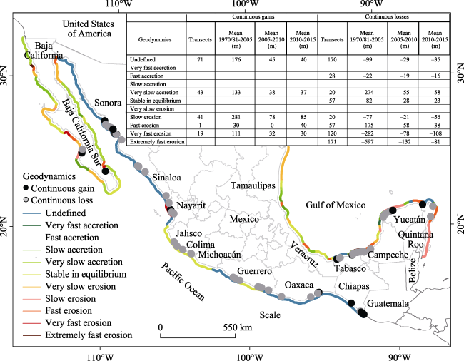
Figure 12 Comparison between sites with continuous unidirectional coastline gains (accretion) and losses (erosion) and the type of geodynamics according to Silva et al. (2014b)
Except for the above-mentioned transects, most coastline transects showing continuous unidirectional processes, of either loss or gain, corresponded to areas described as undefined in the geodynamic processes map (Figure 12). These discrepancies between our map and the geodynamic process map may be due to differences in the scales and temporal context used for elaborating the maps. It must also be considered that Silva et al. (2014b) covered the entire Mexican coast, while we analysed only 66% of it.

4 Conclusions

Coastline change dynamics were monitored for 66% of the Mexican coast between 1970/81 and the present (2015) using data generated by CONABIO´s SMMM. The accuracy of the materials and the methods used were insufficient to describe how coastline changes occurred between the observation periods, but we were able to observe the general trends and to locate zones with dramatic coastline changes. By analysing the types of coastline change (loss or gain) and their dynamics over the observation periods, it was possible to identify coastline segments where continuous dynamic processes took place, to quantify these processes, and to characterize them in order to identify their most probable causes.
Erosion predominated over accretion both in the number of sites and in area affected. In 83% of accretion areas and 73% of erosion areas the type of land cover most affected was Without apparent vegetation, mainly beaches. However, the land cover class of sites showing continuous erosion or accretion dynamics was most often Mangrove (53% of the area showing continuous unidirectional changes), distributed mainly in Campeche and Tabasco (Region 3) and in Nayarit (Region 11). The coastline segments with the highest incidence of net erosive processes were coastal areas with subaerial deposition, mostly consisting of mangroves and beaches, underscoring the fragility of these two ecosystems and the general trend these areas exhibit in erosive processes.
Our analyses underline that processes of erosion and accretion have been accelerating in recent years. The estimated average rates of erosion and accretion for the 2005-2010 and 2010-2015 time periods were twice that of the earliest time period (1970/81-2005), with erosion rates ranging from -3 m/yr to -7.5 m/yr and -7.3 m/yr, and accretion rising from 2.8 m/yr to 7.3 m/yr and 6.9 m/yr, respectively. Further investigation is required to identify the causes of change, which is beyond the scope of our present paper. Potential causes could be synergies between changes in global and regional climatic conditions and increased development of infrastructure, which have modified the coastal dynamics in terms of hydrodynamic processes and sedimentation.
Overall, these results point to the vulnerability of Mexican coastlines and should be made public so that governmental and civil defence decision makers, as well as the population in settlements potentially affected by coastline erosion are aware of the consequences.
The methodology applied in this study helps to identify areas in which coastal management plans should be modified according to their specific coastline change dynamics. However, the need for more in-depth research for monitoring coastline evolution must be underlined. Studies at a multi-scale level, in which in-situ monitoring complements national and regional information, are required to reach a comprehensive understanding of the processes involved in coastal evolution, hence improving coastal management.
[1]
Bird E C F , 1985. Coastline Changes: A Global Review. Chichester, England: John Wiley-Interscience, 219 pp.

[2]
Boak E H, Turner I L , 2005. Shoreline definition and detection: A review. Journal of Coastal Research, 214: 688-703. .

[3]
Cambers G , 1991. Coastlines of the Caribbean, Proc.7th Symposium on Coastal and Ocean Management, Long Beach, Calif., July 8-12, 1991. Amer. Soc. Civil Engnrs, New York, 187 pp.

[4]
Delgadillo-Calzadilla M A, Mendoza E, Silva R et al., 2014. Beach erosion in San Benito Chiapas, Mexico: Assessment and possible solution. Journal of Coastal Research, 71(Suppl.1):114-121.

[5]
Diario Oficial de la Federación de México (2013, December 13) . Programa sectorial de Turismo 2013-2018,Secretaria de Turismo [on line]. Available in: . [2017, September 06].

[6]
Escudero M, Silva R, Mendoza E , 2014. Beach erosion driven by natural and human activity at Isla del Carmen Barrier Island, Mexico. Journal of Coastal Research, 71(Suppl.1):62-74.

[7]
García E , 1988. Modificaciones al sistema de clasificación climática de Koppen. Instituto de Geografía, UNAM, México.

[8]
Goff J, Chague-Goff C, Nichol S et al., 2012. Progress in palaeotsunami research. Sedimentary Geology, 243:70-88.

[9]
Goldenberg S B, Landsea C W, Mestas-Nuñez A M et al., 2001. The recent increase in Atlantic hurricane activity: Causes and implications. Science, 293(5529):474-479.

[10]
Halpern B S, Walbridge S, Selkoe K A et al., 2008. A global map of human impact on marine ecosystems. Science, 319(5865):948-952.

[11]
Hernández-Santana J R, Ortiz-Pérez M A, Linares-Mendez A P et al., 2008. Morfodinámica de la línea de costa del estado de Tabasco, México: Tendencias desde la segunda mitad del siglo XX hasta el presente. Investigaciones Geográficas, Boletín Del Instituto de Geografía,UNAM, ( 65):7-21.

[12]
Hou X Y, Wu T, Hou W et al., 2016. Characteristics of coastline changes in mainland China since the early 1940s. Science China Earth Sciences, 59:1791-1802. doi: 10.1007/s11430-016-5317-5.

[13]
Inman D L, Nordstrom C E , 1971. On the tectonic and morphological classification of cloasts. Journ. of Geol., 79:1-21.

[14]
IPCC, 2007. Climate change 2007: Calcium carbonate structures declines (S22) C. (eds.). Contribution of Working Group II to the Fourth Assessment Report of the Intergovernmental Panel on Climate Change. Published for the Intergovernmental Panel on Climate Change. Cambridge University Press.

[15]
Juanes J L, Ramirez E, Caballero M et al., 1986. Dinámica de los sedimentos en la peninsula de Hicacos, Cuba. II. Efecto de las olas de viento en la zona costera. Revista: Ciencias de la tierra y del espacio, Nº11.

[16]
Kunkel K E, Karl T R, Brooks H et al., 2012. Monitoring and Understanding Trends in Extreme Storms: State of Knowledge. 2012 American Meteorological Society, 57pp.

[17]
Landsea C W, Pielke Jr R A, Mestas-Nunez A M et al., 1999. Atlantic basin hurricanes: Indices of climatic changes. Climatic Change, 42(1):89-129.

[18]
Leatherman S P , 1988. Beach response strategies to accelerated sea level rise. Proceedings 2nd North American Conference on Preparing for Climate Change, The Climate Institute, Washington, D.C. 353-358.

[19]
Lovelock C E, Feller I C, Ellis J et al., 2007. Mangrove growth in New Zealand estuaries: The role of nutrient enrichment at sites with contrasting rates of sedimentation. Oecologia, 153(3):633-641.

[20]
Martell R, Mariño I, Mendoza E G et al., 2010a. Variaciones morfológicas a largo plazo del perfil de playa en Cancún, México. Memorias del xxi Congreso Nacional de Hidráulica, Guadalajara, Jalisco, México, Octubre 2010. 8pp.

[21]
Martell R, Mariño I, Mendoza E G et al., 2010b. Evolución morfodinámica 2D de las playas de Cancún y Puerto Morelos, estado de Quintana Roo, México, V Congreso Latinoamericano de Hidráulica Punta del Este, Uruguay, Noviembre 2010, 15p, IAHR.

[22]
Martell R, Mendoza E, Mariño-Tapia I , et al., 2012. Impactos de corto plazo del huracán Dean sobre la morfología de la playa de Cancún, México. Tecnología y Ciencias del Agua, 3(4):89-111.

[23]
Martínez Martínez R E, Silva R, Mendoza E , 2014. Identification of coastal erosion causes in Matanchén Bay, San Blas, Nayarit, Mexico. Journal of Coastal Research, 71(Suppl.1):93-99.

[24]
Odériz I, Mendoza E, Leo C et al., 2014. An alternative solution to erosion problems at Punta Bete-Punta Maroma, Quintana Roo. Mexico: Conciliating tourism and nature. Journal of Coastal Research, 71(Suppl.1):75-85.

[25]
Ortíz Pérez M A, Espinosa Rodríguez L M , 1991. Una clasificación geomorfológica de las costas de méxico. Geografía y Desarrollo, 2(6):2-9.

[26]
Ortíz-Pérez M A, de la Lanza-Espino G A , 2006. Diferenciación del espacio costero de México: Un inventario regional. Serie de Textos Universitarios.

[27]
Ortíz-Pérez M A, Méndez Linares A P , 2004. Vulnerabilidad al acenso del nivel del mar y sus implicaciones en las cosas bajas del Golfo de México y Mar Caribe. In: Rivera Arriaga E, Villalobos TG J, I. Azuz Adeath y F. Rosado May (eds.). El manejo Costero en México. Universidad A. de Campeche, SEMARNAT, CETYS-Universidad, Universidad de Quintana Roo, 307-320654.

[28]
Peduzzi P, Chatenoux B, Dao H et al., 2012. Global trends in tropical cyclone risk. Nature Climate Change, 2:289-294.

[29]
Rodríguez-Zúñiga M T, Troche-Souza C, Vázquez-Lule A D et al., 2012. Los manglares de México: estado actualy establecimiento de un programa de monitoreo a largo plazo: 2ª y 3era etapas. Comisión Nacional para el Conocimiento y Uso de la Biodiversidad. Informe final SNIB-CONABIO proyecto No. GQ004. México, D.F.

[30]
Sagarpa, 2015. Annual report to the commission. Part 1: Information on fisheries, research, and statistics. Mexico. 1 pp.

[31]
Sarukhán J et al., 2009. Síntesis. Conocimiento actual, evaluación y perspectivas de sustentabilidad, Capital natual de m éxico.

[32]
Sectur, 2015. Compendio Estadístico del Turismo en México 2015. Retrieved from: .

[33]
Semar, 2018. Red Mereográfica Nacional de la Secretaría de Marina. Retrieved from: .

[34]
Silva R, Mariño I Enriquez C , et al., 2006. Monitoring shoreline changes at Cancun beach, Mexico: Effects of Hurricane Wilma. World Scientific Publishing, ICCE Coastal Engineering, Vol. 4:3491-3503.

[35]
Silva R, Martínez M L, Hesp P A et al., 2014 a. Present and future challenges of coastal erosion in Latin America. Journal of Coastal Research, 71(Suppl.1):1-16.

[36]
Silva R, Villatoro M, Ramos F et al., 2014b. Caracterización de la zona costera y planteamiento de elementos técnicos para la elaboración de criterios de regulación y manejo sustentable. Instituto de ingeniería UNAM y SEMARNAT. 177 pp.

[37]
Shepard F P , 1963. Submarine Geology.2nd ed. New York: Harper and Row, 557 pp.

[38]
Thieler E R, Himmelstoss E A, Zichichi J L et al., 2009. The Digital Shoreline Analysis System (DSAS) Version 4.0: An ArcGIS Extension for Calculating Shoreline Change. US Geological Survey.

[39]
Valderrama L, Troche C Rodriguez M T , et al., 2014. Evaluation of mangrove cover changes in Mexico during the 1970-2005 period. Wetlands, 34(4): 747-758. .

[40]
Weinkle J, Maue R, Pielke R Jr , 2012. Historical global tropical cyclone landfalls. Journal of Climate, 25:4729-4735.

[41]
Wentworth C K , 1922. A scale of grade and class terms for clastic sediments. Journal of Geology, 30:377-392.

[42]
Young I R, Zieguer S, Babanin V , 2011. Global trends in wind speed and wave height. Sciencexpress Report(/www.sciencexpress.org/), N10.1126/science.1197219, 8 pp.

Outlines

/