Research Articles

Spatio-temporal distribution of vascular plant species abundance on Qinghai-Tibet Plateau

  • FAN Zemeng 1, 2, 3 ,
  • BAI Ruyu 1, 2 ,
  • YUE Tianxiang 1, 2, 3
Expand
  • 1. State Key Laboratory of Resources and Environment Information System, Institute of Geographic Sciences and Natural Resources Research, CAS, Beijing 100101, China
  • 2. University of Chinese Academy of Sciences, Beijing 100049, China
  • 3. Jiangsu Center for Collaborative Innovation in Geographical Information Resource Development and Application, Nanjing 210023, China

Fan Zemeng, PhD, specialized in ecological modelling and system simulation. E-mail: fanzm@lreis.ac.cn

Received date: 2017-06-20

  Accepted date: 2018-02-27

  Online published: 2019-12-09

Supported by

National Key R&D Program of China(No.2017YFA0603702)

National Key R&D Program of China(No.2018YFC0507200)

National Natural Science Foundation of China(No.41271406)

National Natural Science Foundation of China(No. 91325204)

Innovation Project of LREIS(O88RA600YA)

Copyright

Copyright reserved © 2019. Office of Journal of Geographical Sciences All articles published represent the opinions of the authors, and do not reflect the official policy of the Chinese Medical Association or the Editorial Board, unless this is clearly specified.

Abstract

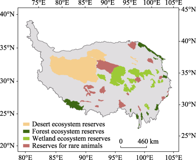
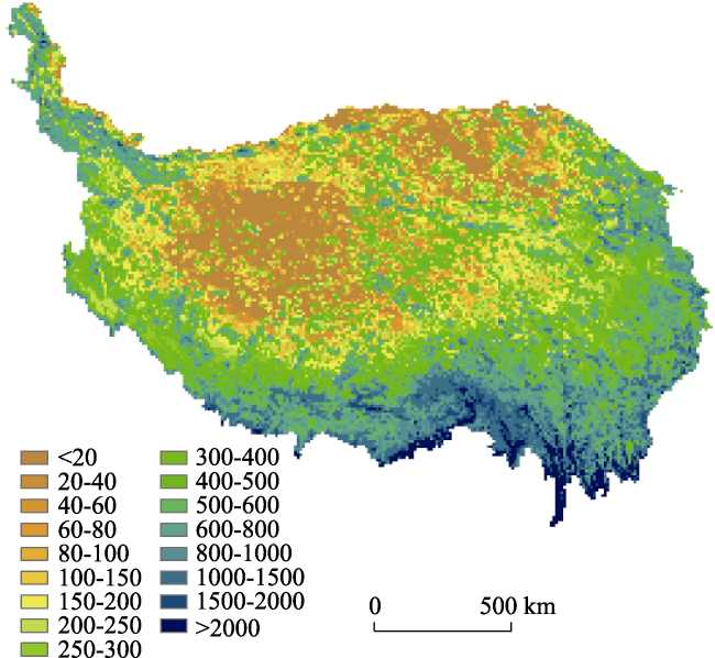
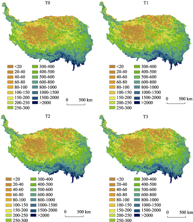
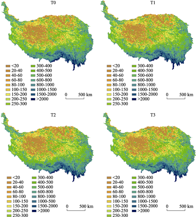
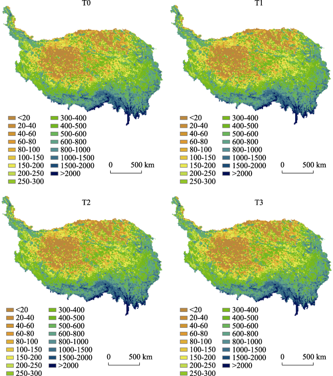
For quantitatively explaining the correlations between the vascular plant species abundance (VPSA) and habitat factors, a spatial simulation method has been developed to simulate the distribution of VPSA on the Qinghai-Tibet Plateau. In this paper, the vascular plant type, land cover, mean annual biotemperature, average total annual precipitation, topographic relief, patch connectivity and ecological diversity index were selected to screen the best correlation equation between the VPSA and habitat factors on the basis of 37 national nature reserves on the Qinghai-Tibet Plateau. The research results show that the coefficient of determination between VPSA and habitat factors is 0.94, and the mean error is 2.21 types per km2. The distribution of VPSA gradually decreases from southeast to northwest, and reduces with increasing altitude except the desert area of Qaidam Basin. Furthermore, the scenarios of VPSA on the Qinghai-Tibet Plateau during the periods from 1981 to 2010 (T0), from 2011 to 2040 (T2), from 2041 to 2070 (T3) and from 2071 to 2100 (T4) were simulated by combining the land cover change and the climatic scenarios of CMIP5 RCP2.6, RCP4.5 and RCP8.5. The simulated results show that the VPSA would generally decrease on the Qinghai-Tibet Plateau from T0 to T4. The VPSA has the largest change ratio under RCP8.5 scenario, and the smallest change ratio under RCP2.6 scenario. In general, the dynamic change of habitat factors would directly affect the spatial distribution of VPSA on the Qinghai-Tibet Plateau in the future.

Cite this article

FAN Zemeng , BAI Ruyu , YUE Tianxiang . Spatio-temporal distribution of vascular plant species abundance on Qinghai-Tibet Plateau[J]. Journal of Geographical Sciences, 2019 , 29(10) : 1625 -1636 . DOI: 10.1007/s11442-019-1667-1

1 Introduction

Vascular plants can provide the necessary material and energy for other species, so the spatial distribution of vascular plant and its abundance directly affects other species structure distribution and diversity (Gaston et al., 2000). Vascular plants play an important role between climate and atmosphere by intercepting water and nutrient cycling to affect soil and water conservation and surface element cycling (Yue et al., 2011; Godínez-Alvarez et al., 2009; Pielke et al., 1998). Long-term interaction between climatic factors, environmental factors and landscape pattern directly controls the spatial distribution of vascular plant species.
How to analyze the spatial distribution pattern of vascular plant species abundance (VPSA), especially simulating the VPSA on a large scale from scattered local survey data, and quantitatively explain the spatial pattern changes of VPSA according to various influencing factors, which has gradually become one of the key issues of biodiversity research field (Gaston et al., 2000; Foley et al., 2005; Kunin et al., 2018). In recent decades, there are many studies on the relationship between spatial distribution of vascular plants and climate change (Zhou et al., 1996). For instance, the changes of temperature and precipitation are the major climate factors affecting the species and distribution of vascular plants (Graham et al., 1990; Stephenson, 1990; Gavilán et al., 2005). Land cover, as the main carrier of global change, directly affects the biological diversity of the earth system (Kalnay et al., 2003; Turner et al., 2007; Rounsevell et al., 2009). For terrestrial ecosystems, land cover change has become one of the main driving factors leading to the species diversity loss and the spatial pattern change of VPSA (Sala et al., 2000; Moreira et al., 2012). The Generalized Additive Models (GAM) was developed to simulate the vegetation distribution in the area of 2600 km2 in western New South Wales, Australia (Zerger et al., 2009). The BIOME4 model was used to simulate the geographical distribution of vegetation types in the Tibetan Plateau (Song et al., 2005). A prediction model of vegetation type distribution was developed by combining the community-habitat regression analysis and geographical information technology on the basis of sample survey data (Shen et al., 2007).
The Qinghai-Tibet Plateau is one of the 25 hotspot areas of global biodiversity conservation (Myers et al., 2000; Sun et al., 2012; Zhang et al., 2016), which has the unique natural environmental condition and the large interchange range of different biota. Based on the method of remote sensing and geographical information technology, many studies have been done on the spatial distribution of vegetation in terms of ecological and environmental driving factors of the Qinghai-Tibet Plateau. For instance, Zhang et al. (2016) quantitatively assessed the changes of net primary productivity (NPP) of nature reserves based on large-scale sampling and comparison methods. Zhuo et al. (2010) analyzed the vegetation changing trends by using remote sensing data from 2000 to 2007. Liao et al. (2014) analyzed the relationship between the topographic factor and elevation, and estimated the vegetation changes in the eastern agricultural region of Qinghai Province from 2000 to 2009. Zhong et al. (2010) used the SPOT vegetation data from 1998 to 2006 to explain the vegetation change, and found that there exists a significant relationship between the vegetation distribution and climatic change. The vegetation area had shown a fluctuated changing trend from 1982 to 2002 (Zhou et al., 2007), and had increased from 2000 to 2009 (Zhang et al., 2013). The vegetation growth in spring showed an increasing trend before 1999, and then appeared a delay change trend during the period from 1982 to 2006 (Piao et al., 2011). Wang et al. (2014) discussed the spatial characteristics of vegetation change and its relationship with climatic factors at different time scales. Liu et al. (2013) found that there was a positive correlation between temperature and vegetation area by combining the vegetation cover data and climatic data from 1981 to 2005.
The current researches mainly focused on simulating the changing trend of vegetation types and land cover of the Qinghai-Tibet Plateau, and counting the VPSA at the local area scale on the basis of sampling data. How to simulate the VPSA distribution is rarely involved by extending the scatter observation data (Crist et al., 2000; Foley et al., 2005; Wade et al., 2011). Therefore, the paper aims to use the VPSA sample data coming from 37 national nature reserves located on the Qinghai-Tibet Plateau, combine the land cover data, climatic factors (mean annual biotemperature and average total annual precipitation), terrain elements, and the landscape indexes (landscape ecological diversity and landscape patch connectivity), and then develop the spatial simulation model for simulating the VPSA distribution change of the Qinghai-Tibet Plateau.

2 Data and methods

2.1 Datasets

The current land cover data in 2010 with a spatial resolution of 1 km × 1 km on the Qinghai-Tibet Plateau has been extracted from the land cover data of whole China (Liu et al., 2014). The land cover scenario data in 2040 (T1), 2070 (T2) and 2010 (T3) with a spatial resolution of 1 km × 1 km has been obtained by operating the surface model of land cover in CMIP5 RCP2.6, RCP4.5 and RCP8.5 scenarios (Fan et al., 2005; Yue et al., 2005; 2007; Yue, 2011; Fan et al., 2015). The climatic data with a spatial resolution of 1 km × 1 km has been simulated by a high accuracy and speed method of surfacing modeling (HASM), including the mean annual biotemperature and average total annual precipitation from 1981 to 2010, and the climatic scenarios raster data in the RCP2.6, RCP4.5 and RCP8.5 of CMIP5 from T1 to T3 (Yue and Wang, 2010; Yue, 2011; Fan et al., 2013a; 2013b; Yue et al., 2013). The vascular plant species data has been obtained from the 37 national nature reserves on the Qinghai-Tibet Plateau, which was published by the Ministry of Ecology and Environment of the People’s Republic of China (http://www.zhb.gov.cn/stbh/zrbhq/qgzrbhqml/). The Qinghai-Tibet Plateau boundary data has been obtained from Global Change Research Data Publishing & Repository (Zhang et al., 2002; Zhang et al., 2014) (http://www.geodoi.ac.cn/ doi.aspx?doi=10.3974/geodb.2014.01.12.v1). The boundary map of the protected area was collected from the Ministry of Ecology and Environment of the People’s Republic of China, and digitized manually within ArcGIS software (Yue et al., 2001; Fan et al., 2013b) (Figure 1). The DEM data were from NASA’s SRTM (http://srtm. csi.cgiar.org/) with a spatial resolution of 1 km × 1 km.
Figure 1 Spatial distribution of national nature reverses on the Qinghai-Tibet Plateau

2.2 Model parameters

The current results show that the intensity of land cover change in national nature reserves is lower than that in non-protected areas (Fan et al., 2013b). The spatial distribution of the VPSA in national nature reserves has a good correlation with mean annual biotemperature, average total annual precipitation, topographic relief, land cover pattern. So, the vascular plant species data of national nature reserve on the Qinghai-Tibet Plateau are used to develop the spatial simulation method of VPSA. The land cover, climatic factors, topographic relief, and landscape index have been selected to analyze the spatial correlation between the spatial distribution of the VPSA and habitat factors on the Qinghai-Tibet Plateau.
First of all, the area of each land cover type (including: cultivated land, forest, grassland, wetland, built-up land, desert and bare rock, snow and ice) has been computed by operating GIS software.
Secondly, the spatial correlation between VPSA and environmental factors has been analyzed in terms of the mean annual biotemperature (MAB), average total annual precipitation (TAP) (Fan et al., 2015), and topographic relief (RE). The calculation equations of MAB, TAP and RE formula can be respectively formulated as:
$MAB\left( x,y \right)=\frac{1}{365}\underset{j=1}{\overset{365}{\mathop \sum }}\,TE{{M}_{>0}}\left( j,x,y,t \right)$
$TAP\left( x,y \right)=\underset{j=1}{\overset{365}{\mathop \sum }}\,P\left( j,x,y \right)$
$Re=\frac{{{A}'}}{A}$
where MAB(x, y) represents the value of MAB at site (x, y); TEM>0 (j, x, y, t) represents the value summing the hourly temperature above 0℃ on the jth day and being divided by 24; TAP(x, y) represents the value of average total annual precipitation at site (x, y); P(j, x, y) represents the mean of precipitation at site (x, y) on the jth day; Re is the topographic relief; A' is the area of the true terrain surface, and A is the area of the terrain projection on the plane.
Moreover, the ecological diversity index and patch connectivity index of land cover (Yue, 1999; Yue and Liu, 2004; Fan et al., 2005; Van Vuuren et al., 2011) have been selected to analyze the correlation between VPSA and landscape index, which can be respectively formulated as:
$D\left( t \right)=\frac{ln{{\left( \mathop{\sum }_{i=1}^{m\left( \varepsilon \right)}{{\left( {{p}_{i}}\left( t \right) \right)}^{1/2}} \right)}^{2}}}{ln\left( \varepsilon \right)}$
$Co(t)=\sum\limits_{i=1}^{m(t)}\sum\limits_{j=1}^{n(t)}P_{ij}(t)S_{ij}(t)$
$S_{ij}(t)=\frac{8\sqrt{3}A_{ij}(t)}{(pr_{ij}(t))^{2}}$
where t is the variable of time; D(t) and m(ε) are respective.ly the ecological diversity of land cover and the total number of the land cover type; Pi(t) is the probability of the ith land cover type of the total study area; ε=(e+a)-1 is the observation scale, a is the total area of land cover, e equals 2.71828; Co(t) is the patch connectivity of land cover; Aij(t) is the area of the jth patch in the ith land cover type; prij(t) is the perimeter of the jth patch in the ith land cover type; $8\sqrt{3}$ is the ratio of the square of perimeter to the area of a hexagon; m(t) is the number of land cover type, n(t) is the patch number of a certain land cover type; Pij(t) is the proportional area of the jth land cover patches to the total area of the ith land cover type.
Finally, on the basis of the basic data of VPSA from the 37 national nature reserves on the Qinghai-Tibet Plateau, land cover, MAB, TAP and landscape index, the correlations between habitat factors and VPSA are analyzed, and the optimal regression equations are selected.
The linear regression and non-linear regression models have been generally adopted to create the current species-area curve and other species abundance models, but the selected model format has many limitations. For overcoming them, the linear model (y=A+Bx), logarithmic model (y=A+Blnx) and exponential model (y=Bex) were respectively used. Where y represents the VPSA, x represents the influencing factor, and A and B are fitted coefficients. The regression models and fitted coefficients between VPSA and explanatory variables are summarized in Table 1.
Table 1 Equations between vascular plant abundance and driving factors
Factor type Function type Equation Coefficient of determination
Environ- ment
variable
Linear $y=259.79+120.06MAB-0.31MAP+3179.40Re$ R=0.85
Exponent and logarithm $y=-756.85+0.20exp(MAB)-118.68lnMAP+1950.94exp(Re)$ R=0.91
Logarithm $y=-2789.60-25.10lnMAB-665.62lnMAP+395.03lnRe$ R=0.68
Landscape index Linear $y=1217.50-1643.47Cot+3245.51Dt$ R=0.31
Exponent $y=-541.70-1547.10exp\left( Cot \right)+3301.28exp\left( Dt \right)$ R=0.52
Logarithm $y=1109.06+12.06lnCot-38.37lnDt$ R=0.20
Land cover type Linear $\begin{matrix} & y=881.86+2.94*{{10}^{-6}}Ca+7.30*{{10}^{-7}}Fo+1.85*{{10}^{-9}}Gr-7.88* \\ & \ \ \ \ \ \ {{10}^{-9}}Wa-1.61*{{10}^{-4}}Bu-2.17*{{10}^{-8}}De-6.47*{{10}^{-8}}Ic \\ \end{matrix}$ R=0.65
Logarithm $\begin{matrix} & y=388.46+39.83lnCa+57.89lnFo-7.48lnGr-62.01lnWa \\ & \ \ \ \ \ \ -19.96lnBu+2.84lnDe+44.84lnIc \\ \end{matrix}$ R=0.80

Notes: y is the VPSA; MAB, MAP and Re are respectively mean annual biotemperature, total annual average precipitation and topographic relief; Dt and Cot are respectively landscape diversity and patch connectivity of land cover; Ca, Fo, Gr, Wa, Bu, De and Ic are respectively cultivated land, forest land, grassland, wetland, built-up land, desertification land and ice area.

Table 1 shows that the exponent and logarithmic mixed model (R=0.91) is superior to the simple linear model (R = 0.85) and the logarithmic model (R = 0.68) for counting the correlation between environmental factors and VPSA. The exponential model (R = 0.52) is superior to the linear model (R = 0.31) and logarithmic model (R = 0.20) for counting the correlation between landscape index and VPSA. For computing the correlation between the land cover type factor and vascular plant species abundance, the logarithmic model (R = 0.80) is better than other regression format.

2.3 Spatial simulation method of vascular plant species abundance

According to the regression model analysis results of the VPSA and habitat factors, the relationship between the VPSA and land cover type factors, environmental factors and landscape index was analyzed. The three best suitable equations of logarithmic model, exponential logarithmic model and exponential model are used respectively, and then the spatial simulation model of the VPSA distribution on the Qinghai-Tibet Plateau can be formulated as:
$\begin{matrix} & VPSA{{\left( x,y \right)}_{t}}=Cons+{{\omega }_{1}}\left[ \begin{matrix} {{\alpha }_{1}}\ln Ca{{\left( x,y \right)}_{t}} \\ +{{\alpha }_{2}}\ln Fo{{\left( x,y \right)}_{t}} \\ +~{{\alpha }_{3}}\ln Gr{{\left( x,y \right)}_{t}} \\ +~~{{\alpha }_{4}}\ln Wa{{\left( x,y \right)}_{t}} \\ +{{\alpha }_{5}}\ln Bu{{\left( x,y \right)}_{t}} \\ +{{\alpha }_{6}}\ln De{{\left( x,y \right)}_{t}} \\ +{{\alpha }_{7}}\ln Ic{{\left( x,y \right)}_{t}} \\ \end{matrix} \right]+ \\ & \ \ \ \ \ \ \ \ \ \ \ \ \ \ \ \ \ \ \ \ \ {{\omega }_{2}}\left\{ \begin{matrix} {{\beta }_{1}}\exp \left[ MAB{{\left( x,y \right)}_{t}} \right] \\ +{{\beta }_{2}}\ln MAP{{\left( x,y \right)}_{t}} \\ +~{{\beta }_{3}}\exp \left[ Re{{\left( x,y \right)}_{t}} \right] \\ \end{matrix} \right\}+{{\omega }_{3}}\left\{ \begin{matrix} {{\gamma }_{1}}\exp \left[ Cot{{\left( x,y \right)}_{t}} \right] \\ +{{\gamma }_{2}}\exp \left[ Dt{{\left( x,y \right)}_{t}} \right] \\ \end{matrix} \right\} \\ \end{matrix}$
where t is the variable of time; (x, y) is the position coordinate; Cons is constant; ω is the model coefficient; VPSA(x, y)t is the VPSA at site (x, y) in the t period; MAB(x, y)t is the mean annual biotemperature at site (x, y) in the t period; MAP(x, y)t is the average total annual precipitation at site (x, y) in the t period; Re(x, y)t is the average topographic relief at site (x, y) in the t period; Cot(x, y)t is the patch connectivity of land cover at site (x, y) in the t period; Dt(x, t)t is the ecological index at site (x, y) in the t period; Ca(x, y)t is the area of cultivated land at site (x, y) in the t period; Fo(x, y)t is the area of forest at site (x, y) in the t period; Gr(x, y)t is the area of grassland at site (x, y) in the t period; Wa(x, y)t is the area of water at site (x, y) in the t period; Bu(x, y)t is the area of built-up land at site (x, y) in the t period; De(x, y)t is the area of desert at site (x, y) in the t period; Ic(x, y)t is the area of snow and ice at site (x, y) in the t period; α1, α2, α3, α4, α5, α6 and α7 are the fitted coefficients between the VPSA and the land cover types; β1, β2 and β3 are the fitted coefficients between the VPSA and mean annual biotemperature, average total annual precipitation, and topographic relief; γ1 and γ1 are the fitted coefficients between the VPSA and ecological diversity, and patch connectivity index. The fitted coefficients of explanatory variables in equation (7) are obtained by running the best suitable regression equation of the vascular plant species (Figure1) covering 37 national nature reserves on the Qinghai-Tibet Plateau: Cons = ‒11582.89, ω1 = 0.38, ω2 = 0.98, ω3 = 1.02, α1 = 66.08, α2 = 0.68, α3 = 2.40, α4 = ‒34.22, α5 = 4.04, α6 = 31.63, α7 = 56.00, β1 = 0.23, β2 = 536.45, β3 = 1400.28, γ1 = ‒283.11, γ2 = 6007.68. The coefficient of determination of equation (7) is R=0.94 and passes the significance test of 0.01. The spatial distribution and scenarios of VPSA on the Qinghai-Tibet Plateau were simulated and analyzed by operating the spatial simulation method of VPSA.

3 Results

3.1 Model validation

The spatial distribution of VPSA was simulated by operating the spatial distribution model of VPSA with the vascular plant species data from the 37 national nature reserves and land cover data in Qinghai-Tibet Plateau in 2010. For validating the model accuracy, the mean VPSA number (per km2) was calculated in each nature reserve. The error between the simulated value of the VPSA number per km2 and the statistical value can be calculated as:
${{S}_{Error}}=\frac{1}{n}\underset{i=1}{\overset{n}{\mathop \sum }}\,\left( \frac{\left| Valu{{e}_{is}}-Valu{{e}_{it}} \right|}{{{S}_{i}}} \right)$
where SError is the simulation error of VPSA, n is the number of nature reserves, Si is the area of the ith nature reserve, Valueis and Valueit respectively represent the simulated value and statistical value of VPSA in the ith national nature reserve.
The error analysis results show that the overall simulation error of VPSA is 2.21 types per km2 in the 37 national nature reserves of the Qinghai-Tibet Plateau. The simulation result has a good accordance with the actual VPSA distribution on the Qinghai-Tibet Plateau, which indicates the developed model of VPSA can be used to simulate the spatial distribution of VPSA on a regional scale.

3.2 Spatial distribution of vascular plants species abundance

According to the spatial distribution of VPSA on the Qinghai-Tibet Plateau (Figure 2), the number of average VPSA is 496.79 species per 100 km2. The VPSA distribution gradually decreased from the southeast towards the northwest. The VPSA of the central-western Qinghai-Tibet Plateau and Qaidam Basin is less than other areas, and the average species abundance of vascular plants is less than 200 species per 100 km2. The high VPSA is mainly distributed in the mountain areas of Minshan-Qionglai-Daxue, Gaoligongshan-Nushan-Yulong, and the transitional zone between the western Qinling and Qilian mountains, where the VPSA number is more than 600 species per 100 km2. Especially in the rivers of Bailong, Dadu, Jinsha, Lancang, Nujiang and Brahmaputra, the VPSA number is up to 1000 species per 100 km2, and even more than 2000 species per 100 km2 in certain local area.
Figure 2 Spatial distribution of VPSA in Qinghai-Tibet Plateau in 2010

3.3 Scenario analysis of vascular plant species abundance

The simulation results of VPSA scenarios (Table 2 and Figures 3-5) show that the VPSA would decrease under three climate change scenarios of the Qinghai-Tibet Plateau from T0 to T4.
Table 2 Changes of VPSA under three scenarios on the Qinghai-Tibet Plateau
Scenarios T0 ∆(T1-T0) T1 ∆(T1-T0) T2 ∆(T1-T0) T3
RCP2.6 496.79 -0.53 496.26 -0.17 496.09 -0.04 496.05
RCP4.5 496.79 0.27 497.06 -1.42 495.64 -1.05 494.59
RCP8.5 496.79 0.52 497.31 -1.95 495.36 -4.15 491.21
Figure 3 Spatial distribution of VPSA under RCP2.6 scenario on the Qinghai-Tibet Plateau
Figure 4 Spatial distribution of VPSA under RCP4.5 scenario on the Qinghai-Tibet Plateau
Figure 5 Spatial distribution of VPSA under RCP8.5 scenario in Qinghai-Tibet Plateau
Under RCP2.6 scenario, the VPSA would show a decreasing trend, but the change ratio would respectively decrease by 0.11%, 0.03% and 0.04% during the three periods from T0 to T1, T1 to T2 and T2 to T3. Under RCP4.5 scenario, the VPSA would increase by 0.05% from T0 to T1, while it would respectively decrease by 0.29% and 0.21% during the two periods from T1 to T2 and from T2 to T3. Under RCP8.5 scenario, the VPSA would increase by 0.10% from T0 to T1, while it would respectively decrease by 0.39% and 0.84% during the two periods from T1 to T2 and from T2 to T3. Under the three scenarios, the change of VPSA would have the maximum change amplitude under RCP8.5 scenario, and then under RCP4.5 scenario, while it is the minimum change amplitude under RCP2.6 scenario of the Qinghai-Tibet Plateau.

4 Discussion and conclusions

The existing investigations about VPSA are mainly focused on statistical analysis in a certain local area or administrative unit in terms of field observation and sample data, but rarely involve the spatial simulation of VPSA on a middle or large scale, and especially on the scenarios simulation of the spatial distribution of VPSA. Moreover, while the correlation between VPSA and habitat factors is computed, the traditional statistical models of VPSA is limited to consider a single driving factor, such as species-area curve method only considers the correlation between species richness and land cover area. For explaining how the multiple habitat factors affect the VPSA distribution, a few integrated models had been developed by combining the climatic change and land cover change, but without taking into account the reaction effect between the ecological landscape complexity and VPSA. In view of the limitations of the existing models, the influencing factors are classified into three types that include land cover factor, environmental factor and landscape index factor, and then a new integrated model has been developed for simulating the spatial distribution of VPSA in terms of the vascular plant data covering 37 national nature reserves on the Qinghai-Tibet Plateau. In this paper, the linear regression function and non-linear regression (logarithmic, exponential) functions are combined to develop the spatial simulation method of VPSA of the Qinghai-Tibet Plateau.
The comparative analysis results between the simulation value of VPSA in 2010 and the biodiversity survey data (Xu et al., 2013) show that the simulated distribution pattern has a good consistent with the actual distribution of VPSA, which indicates that the spatial simulation method of VPSA can be used to simulate the spatial distribution change of VPSA on the Qinghai-Tibet Plateau. The spatial simulation method of VPSA, as an integrated model, can overcome the limitation of existing models which cannot simulate the spatial distribution of VPSA on a middle or large scale. In the process of model development, not only the land cover type and environmental factors are taken into account, but also the landscape index is considered. Furthermore, the spatial simulation method of VPSA can be used to predict the VPSA change under different climatic change scenarios. The simulation results can provide support for estimating the influences of climate change on ecosystem services and biodiversity change.
However, due to lack enough basic data of VPSA, the spatial simulation method of VPSA only consider the data of the published 37 national nature reserves located on the Qinghai-Tibet Plateau. It is required to combine more field sample data of VPSA and high-resolution remote sensing data for improving the simulation accuracy, which is the focal point of our next research works on the spatial simulation method of VPSA.
[1]
Crist P, Kohley T, Oakleaf J , 2000. Assessing land-use impacts on biodiversity using an expert systems tool. Landscape Ecology, 15(1):47-62.

[2]
Fan Z M, Li J, Yue T X , 2013 a. Land-cover changes of biome transition zones in Loess Plateau of China. Ecological Modelling, 252:129-140.

[3]
Fan Z M, Li J, Yue T X et al., 2015. Scenarios of land cover in karst area of southwestern China. Environment Earth Science, 74(1):6407-6420.

[4]
Fan Z M, Yue T X, Liu J Y et al., 2005. Spatial and temporal distribution of land cover scenarios in China. Acta Geographica Sinica, 60(6):63-74. (in Chinese)

[5]
Fan Z M, Zhang X, Li J et al., 2013b. Land-cover changes of national nature reserves in China. Journal of Geographical Sciences, 23(2):258-270.

[6]
Foley J, DeFries R, Asner G et al., 2005. Global consequences of land use. Science, 309(5734):570-574.

[7]
Gaston K , 2000. Global patterns in biodiversity. Nature, 405(6783):220-227.

[8]
Gavilán R , 2005. The use of climatic parameters and indices in vegetation distribution: A case study in the Spanish Sistema Central. International Journal of Biometeorology, 50(2):111-120.

[9]
Godínez-Alvarez H, Herrick J, Mattocks M et al., 2009. Comparison of three vegetation monitoring methods: Their relative utility for ecological assessment and monitoring. Ecological Indicators, 9(5):1001-1008.

[10]
Graham R, Grimm E C , 1990. Effects of global climate change on the patterns of terrestrial biological communities. Trends in Ecology & Evolution, 5(9):289-292.

[11]
Kalnay E, Cai M , 2003. Impact of urbanization and land-use change on climate. Nature, 423(6939):528-531.

[12]
Kunin W E, Harte J, He F L et al., 2018. Upscaling biodiversity: Estimating the species-area relationship from small samples. Ecological Monographs, 88(2):170-187

[13]
Liao Q F, Zhang X, Ma Q Q et al., 2014. Spatiotemporal variation of fractional vegetation cover and remote sensing monitoring in the eastern agricultural region of Qinghai Province. Acta Ecologica Sinica, 34(20):5936-5943. (in Chinese)

[14]
Liu J H, Gao J X, Wang W J , 2013. Variations of vegetation coverage and its relations to global climate changes on the Tibetan Plateau during 1981-2005. Journal of Mountain Science, 31(2):234-242. (in Chinese)

[15]
Liu J Y, Kuang W H, Zhang Z X et al., 2014. Spatiotemporal characteristics, patterns and causes of land use changes in China since the late 1980s. Acta Geographica Sinica, 69(1):3-14. (in Chinese)

[16]
Moreira F, Silva J, Estanque B et al., 2012. Mosaic-level inference of the impact of land cover changes in agricultural landscapes on biodiversity: A case-study with a threatened grassland bird. PloS One, 7(6):38876.

[17]
Myers N, Mittermeier R, Mittermeier C et al., 2000. Biodiversity hotspots for conservation priorities. Nature, 403(6772):853-858.

[18]
Piao S, Wang X, Ciais P et al., 2011. Changes in satellite-derived vegetation growth trend in temperate and boreal Eurasia from 1982 to 2006. Global Change Biology, 17(10):3228-3239.

[19]
Pielke R, Avissar R, Raupach M et al., 1998. Interactions between the atmosphere and terrestrial ecosystems: Influence on weather and climate. Global Change Biology, 4(5):461-475.

[20]
Rounsevell M, Reay D , 2009. Land use and climate change in the UK. Land Use Policy, 26(1):S160-S169.

[21]
Sala O, Chapin F, Armesto J et al., 2000. Global biodiversity scenarios for the year 2100. Science, 287(5459):1770-1774.

[22]
Shary P, Sharaya L, Mitusov A , 2002. Fundamental quantitative methods of land surface analysis. Geoderma, 107(1):1-32.

[23]
Shen Z H, Zhao J , 2007. Prediction of the spatial patterns of species richness based on the plant topography relationship: An application of GAMs approach. Acta Phytoecologica Sinica, 27(3):953-963. (in Chinese)

[24]
Song M, Zhou C, Ouyang H , 2005. Simulated distribution of vegetation types in response to climate change on the Tibetan Plateau. Journal of Vegetation Science, 16(3):341-350. (in Chinese)

[25]
Stephenson N , 1990. Climatic control of vegetation distribution: The role of the water balance. American Naturalist, 135(5):649-670.

[26]
Sun H L, Zheng D, Yao T D et al., 2012. Protection and construction of the national ecological security shelter zone on Tibetan Plateau. Acta Geographica Sinica, 67(1):3-12. (in Chinese)

[27]
Turner B, Lambin E, Reenberg A , 2007. The emergence of land change science for global environmental change and sustainability. Proceedings of the National Academy of Sciences, 104(52):20666-20671.

[28]
Van Vuuren D, Edmonds J, Kainuma M et al., 2011. The representative concentration pathways: An overview. Climatic Change, 109(1/2):5.

[29]
Wade A, Theobald D, Laituri M , 2011. A multi-scale assessment of local and contextual threats to existing and potential US protected areas. Landscape and Urban Planning, 101(3):215-227.

[30]
Wang Q X, Lv S H, Bao Y et al., 2014. Characteristics of vegetation change and its relationship with climate factors in different time-scales on Qinghai-Xizang Plateau. Plateau Meteorology, 33(2):301-312.

[31]
Xu H G, Cao M C Wu J , et al., 2013. Assessment Report of Biodiversity Background in China. Beijing: China Sciences Press. (in Chinese)

[32]
Yue T X , 2011. Surface Modeling: High Accuracy and High Speed Methods. Boca Raton: CRC Press, Taylor & Francis Group.

[33]
Yue T, Fan Z, Chen C et al., 2011. Surface modelling of global terrestrial ecosystems under three climate change scenarios. Ecological Modelling, 222(14):2342-2361.

[34]
Yue T X, Fan Z M, Liu J Y , 2005. Changes of major terrestrial ecosystems in China since 1960. Global and Planetary Change, 48(4):287-302.

[35]
Yue T X, Fan Z M, Liu J Y , 2007. Scenarios of land cover in China. Global and Planetary Change, 55(4):317-342.

[36]
Yue T X, Zhao N, Ramsey R D et al., 2013. Climate change trend in China, with improved accuracy. Climatic Change, 120(1):137-151.

[37]
Zerger A, Gibbons P, Seddon J et al., 2009. A method for predicting native vegetation condition at regional scales. Landscape and Urban Planning, 91(2):65-77.

[38]
Zhang L, Guo H, Ji L et al., 2013. Vegetation greenness trend (2000 to 2009) and the climate controls in the Qinghai-Tibetan Plateau. Journal of Applied Remote Sensing, 7(1):073572.

[39]
Zhang Y L, Hu Z J, Qi W et al., 2016. Assessment of effectiveness of nature reserves on the Tibetan Plateau based on net primary production and the large sample comparison method. Journal of Geographical Sciences, 26(1):27-44.

[40]
Zhang Y L, Li B Y, Zheng D , 2002. A discussion on the boundary and area of the Tibetan Plateau in China. Geographical Research, 21(1):1-8. (in Chinese)

[41]
Zhang Y L, Li B Y, Zheng D , 2014. The data publish of a discussion on the boundary and area of the Tibetan Plateau in China: Geographical information system data of the boundary and area of the Tibetan Plateau in China. Global Change Research Data Publishing & Repository. doi: 10.3974/geodb.2014.01.12.v1.

[42]
Zhong L, Ma Y, Salama M et al., 2010. Assessment of vegetation dynamics and their response to variations in precipitation and temperature in the Tibetan Plateau. Climatic Change, 103(3/4):519-535.

[43]
Zhou D, Fan G, Huang R et al., 2007. Interannual variability of the normalized difference vegetation index on the Tibetan Plateau and its relationship with climate change. Advances in Atmospheric Sciences, 24(3):474-484.

[44]
Zhou G, Zhang X , 1996. Study on Chinese climate-vegetation relationship. Acta Phytoecologica Sinica, 20(2):113-119. (in Chinese)

[45]
Zhuo Ga, Li Xin, Luo Bu et al., 2010. Dynamical analysis of recent vegetation variation with satellite dataset in Tibet region. Plateau Meteorology, 29(3):563-571. (in Chinese)

Outlines

/