
Journal of Geographical Sciences >
Exploring the database of a soil environmental survey using a geo-self-organizing map: A pilot study
|
Liao Xiaoyong (1977-), PhD and Professor, specialized in evaluation and remediation of soil pollution. E-mail: liaoxy@igsnrr.ac.cn |
Received date: 2018-07-05
Accepted date: 2018-10-31
Online published: 2019-12-09
Supported by
Strategic Priority Research Program of the Chinese Academy of Sciences(No.XDA19040302)
The Key Research Program of the Chinese Academy of Sciences(No.KFZD-SW-111)
Copyright
A model integrating geo-information and self-organizing map (SOM) for exploring the database of soil environmental surveys was established. The dataset of 5 heavy metals (As, Cd, Cr, Hg, and Pb) was built by the regular grid sampling in Hechi, Guangxi Zhuang Autonomous Region in southern China. Auxiliary datasets were collected throughout the study area to help interpret the potential causes of pollution. The main findings are as follows: (1) Soil samples of 5 elements exhibited strong variation and high skewness. High pollution risk existed in the case study area, especially Hg and Cd. (2) As and Pb had a similar topological distribution pattern, meaning they behaved similarly in the soil environment. Cr had behaviours in soil different from those of the other 4 elements. (3) From the U-matrix of SOM networks, 3 levels of SEQ were identified, and 11 high risk areas of soil heavy metal-contaminated were found throughout the study area, which were basically near rivers, factories, and ore zones. (4) The variations of contamination index (CI) followed the trend of construction land (1.353) > forestland (1.267) > cropland (1.175) > grassland (1.056), which suggest that decision makers should focus more on the problem of soil pollution surrounding industrial and mining enterprises and farmland.
Key words: self-organizing map; geo-information; heavy metal; soil environmental quality; Hechi
LIAO Xiaoyong , TAO Huan , GONG Xuegang , LI You . Exploring the database of a soil environmental survey using a geo-self-organizing map: A pilot study[J]. Journal of Geographical Sciences, 2019 , 29(10) : 1610 -1624 . DOI: 10.1007/s11442-019-1644-8
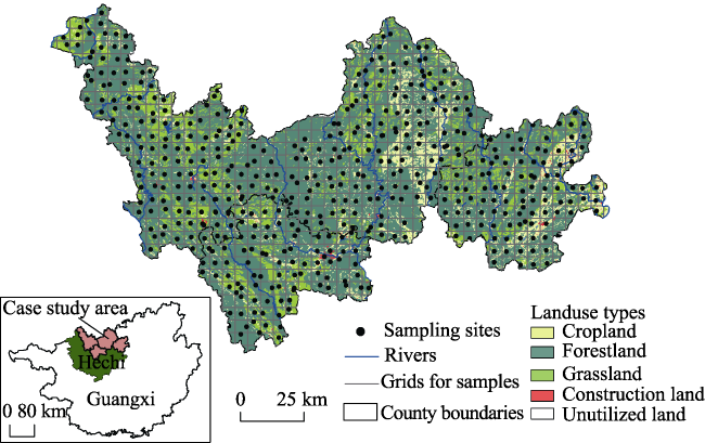
Figure 1 Soil sampling in Hechi, Guangxi Zhuang Autonomous Region in southern China |
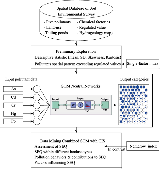
Figure 2 Flowchart of G-SOM for exploring the spatial database of the soil environmental survey |
Table 1 Sample data statistics in Hechi region |
| Elements | Mean (mg·kg-1) | Standard deviation (mg·kg-1) | Variation coefficient (%) | Skewness | Kurtosis | Chinese standard (mg·kg-1) | Exceeding rate (%) |
|---|---|---|---|---|---|---|---|
| As | 27.05 | 94.86 | 351 | 16.03 | 297.07 | 15 | 42.69 |
| Cd | 1.47 | 4.11 | 280 | 9.15 | 123.09 | 0.2 | 51.85 |
| Cr | 68.27 | 56.86 | 83 | 2.25 | 9.83 | 90 | 21.25 |
| Hg | 0.48 | 0.72 | 150 | 5.20 | 39.84 | 0.15 | 73.88 |
| Pb | 76.06 | 192.39 | 250 | 8.50 | 84.73 | 35 | 62.00 |
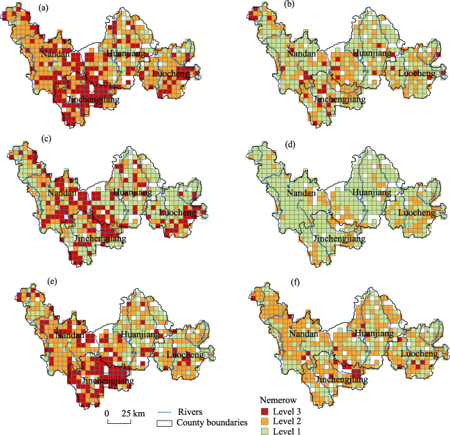
Figure 3 Spatial patterns of soil heavy metal pollution of the Nemerow pollution index map (a), and single-factor index maps of As (b), Cd (c), Cr (d), Hg (e), and Pb (f), respectively |
Table 2 Summary of SOM quality measures |
| Rows | Columns | Map size | Variable | Log | Range | |||
|---|---|---|---|---|---|---|---|---|
| QE | TE | QE | TE | QE | TE | |||
| 11 | 8 | 88 | 0.47 | 0.02 | 0.62 | 0.03 | 0.04 | 0.11 |
| 12 | 8 | 96 | 0.46 | 0.01 | 0.60 | 0.02 | 0.04 | 0.11 |
| 11 | 9 | 99 | 0.45 | 0.02 | 0.60 | 0.04 | 0.04 | 0.15 |
| *13 | *8 | *104 | 0.45 | 0.03 | 0.59 | 0.03 | *0.04 | *0.06 |
| 12 | 9 | 108 | 0.44 | 0.02 | 0.58 | 0.04 | 0.04 | 0.12 |
| 11 | 10 | 110 | 0.44 | 0.03 | 0.58 | 0.04 | 0.04 | 0.18 |
| 13 | 9 | 117 | 0.43 | 0.02 | 0.57 | 0.04 | 0.04 | 0.08 |
| 12 | 10 | 120 | 0.43 | 0.02 | 0.56 | 0.04 | 0.04 | 0.14 |
| 11 | 11 | 121 | 0.42 | 0.03 | 0.56 | 0.03 | 0.04 | 0.17 |
| 13 | 10 | 130 | 0.42 | 0.02 | 0.55 | 0.03 | 0.03 | 0.14 |
| 12 | 11 | 132 | 0.42 | 0.02 | 0.55 | 0.03 | 0.03 | 0.18 |
| 13 | 11 | 143 | 0.41 | 0.02 | 0.54 | 0.03 | 0.03 | 0.15 |
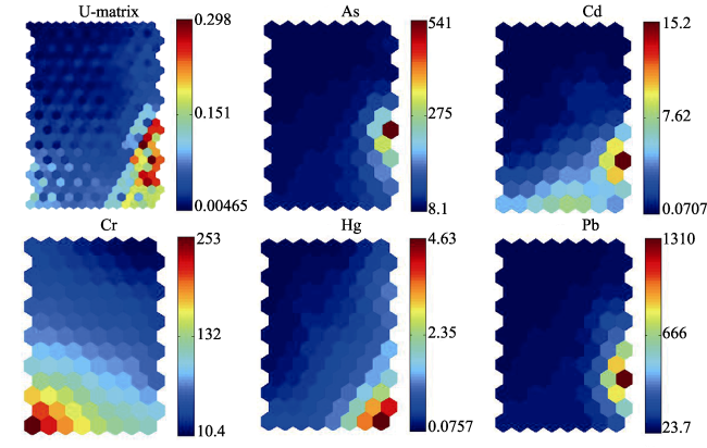
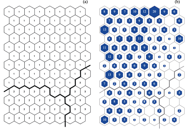
Figure 4 U-matrix of SOM and C-Planes for the five heavy metals (As, Cd, Cr, Hg, and Pb) |
Figure 5 Results of SOM clustering of the categories map of the entire output space (a), and the map of neuronal BMU (b) |
Table 3 Classification statistics of SOM clusters |
| SEQ | Mean content of elements (mg·kg-1) | Counts | | ||||
|---|---|---|---|---|---|---|---|
| As | Cd | Cr | Hg | Pb | |||
| Level 1 | 16.74 | 0.46 | 47.1 | 0.33 | 47.24 | 413 | 2.85 |
| Level 2 | 27.52 | 3.94 | 169.1 | 0.66 | 69.17 | 84 | 15.18 |
| Level 3 | 290.04 | 8.9 | 86.88 | 3.29 | 782.23 | 16 | 49.76 |
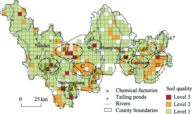
Figure 6 Spatial distribution of SEQ and 4 categories of high-risk areas of mining areas, flood areas, higher natural background value areas and sewage irrigated areas |
Table 4 SEQ for different land-use types published in 2015 |
| Land-use types | SEQ | Counts | CI | ||
|---|---|---|---|---|---|
| Level 1 | Level 2 | Level 3 | |||
| Construction land | 36 (70.6%) | 12 (23.5%) | 3 (5.9%) | 51 | 1.353 |
| Cropland | 167 (86.1%) | 20 (10.3%) | 7 (3.6%) | 194 | 1.175 |
| Forestland | 176 (75.9%) | 50 (21.6%) | 6 (2.6%) | 232 | 1.267 |
| Grassland | 34 (94.4%) | 2 (5.6%) | 0 (0%) | 36 | 1.056 |
| [1] |
|
| [2] |
|
| [3] |
|
| [4] |
|
| [5] |
|
| [6] |
|
| [7] |
|
| [8] |
|
| [9] |
|
| [10] |
|
| [11] |
|
| [12] |
|
| [13] |
|
| [14] |
|
| [15] |
|
| [16] |
|
| [17] |
|
| [18] |
|
| [19] |
|
| [20] |
|
| [21] |
|
| [22] |
|
| [23] |
|
| [24] |
|
| [25] |
|
| [26] |
|
| [27] |
|
| [28] |
|
| [29] |
|
| [30] |
|
| [31] |
|
| [32] |
|
| [33] |
|
| [34] |
|
| [35] |
|
| [36] |
|
/
| 〈 |
|
〉 |