Research Articles

The impact of economic agglomeration on water pollutant emissions from the perspective of spatial spillover effects

  • ZHOU Kan 1 ,
  • LIU Hanchu , 2 ,
  • WANG Qiang 3
Expand
  • 1. Institute of Geographic Sciences and Natural Resources Research, Key Laboratory of Regional Sus-tainable Development Modeling, CAS, Beijing 100101, China
  • 2. Institute of Science and Development, CAS, Beijing100190, China
  • 3. School of Geographical Sciences, Fujian Normal University, Fuzhou 350007, China
Liu Hanchu, PhD, E-mail:

Zhou Kan (1986─), PhD and Associate Professor, specialized in resources and environmental carrying capacity and regional sustainable development. E-mail: zhoukan2008@126.com

Received date: 2019-05-08

  Accepted date: 2019-07-09

  Online published: 2019-12-06

Supported by

The Strategic Priority Research Program of the Chinese Academy of Sciences, No(XDA23020101)

National Natural Science Foundation of China, No(41971164)

National Natural Science Foundation of China, No(41671126)

Copyright

Copyright reserved © 2019. Office of Journal of Geographical Sciences All articles published represent the opinions of the authors, and do not reflect the official policy of the Chinese Medical Association or the Editorial Board, unless this is clearly specified.

Abstract

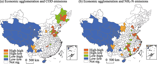
Whether economic agglomeration can promote improvement in environmental quality is of great importance not only to China’s pollution prevention and control plans but also to its future sustainable development. Based on the COD (Chemical Oxygen Demand) and NH3-N (Ammonia Nitrogen) emissions Database of 339 Cities at the city level in China, this study explores the impact of economic agglomeration on water pollutant emissions, including the differences in magnitude of the impact in relation to city size using an econometric model. The study also examines the spillover effect of economic agglomeration, by conducting univariate and bivariate spatial autocorrelation analysis. The results show that economic agglomeration can effectively reduce water pollutant emissions, and a 1% increase in economic agglomeration could lead to a decrease in COD emissions by 0.117% and NH3-N emissions by 0.102%. Compared with large and megacities, economic agglomeration has a more prominent effect on the emission reduction of water pollution in small- and medium-sized cities. From the perspective of spatial spillover, the interaction between economic agglomeration and water pollutant emissions shows four basic patterns: high agglomeration-high emissions, high agglomeration-low emissions, low agglomeration-high emissions, and low agglomeration-low emissions. The results suggest that the high agglomeration-high emissions regions are mainly distributed in the Beijing-Tianjin-Hebei region, Shandong Peninsula, and the Harbin-Changchun urban agglomeration; thus, local governments should consider the spatial spillover effect of economic agglomeration in formulating appropriate water pollutant mitigation policies.

Cite this article

ZHOU Kan , LIU Hanchu , WANG Qiang . The impact of economic agglomeration on water pollutant emissions from the perspective of spatial spillover effects[J]. Journal of Geographical Sciences, 2019 , 29(12) : 2015 -2030 . DOI: 10.1007/s11442-019-1702-2

1 Introduction

In the past 40 years, high-speed and ultra-high-speed economic growth has put increasing pressure on China’s environmental system (Wang et al., 2018; Liang and Yang, 2019). In particular, the carrying capacity of the water environment has reached, or approached, the upper limit (Chen et al., 2018a). By 2016, the quality of some rivers in China continued to deteriorate. For example, because of the high degree of economic and population agglomeration in the Haihe River Basin, the water environment in northern China was seriously polluted, and the proportion of inferior V water quality sections accounted for 35.7% of the whole region (Zhao, 2017). Some rivers flowing through urban areas have a heavily polluted water body that is black and smelly due to a lack of oxygen, which has caused many complaints from the public (Ji et al., 2017). The problem of water pollution seriously restricts improvement in the quality of human settlements and poses a threat to the health of residents (Hu and Cheng, 2013). To solve the problem of environmental capacity overload, it is necessary not only to increase environmental protection and rectification, but also to transform the traditional mode of economic development driven by pollution-intensive industries (Lu, 2015; Fang et al., 2017). Therefore, it is important to fully understand the coupling relationship between economic development and environmental pollution, and to systematically analyze the impact of economic agglomeration on water pollutant emissions. In this regard, this paper not only provides a reference for comprehensive measures against water pollution but also forms a sound basis for environmentally friendly development.
At present, with regard to the relationship between economic growth and pollutant emissions, scholars have conducted extensive investigations from different perspectives that have focused on the impacts of the factors driving pollutant emissions, including the level of economic development, economic structure, foreign trade performance, capital investment, and household consumption. The relationship between economic growth and pollutant emissions generally presents an “inverted U-shaped” curve (Grossman and Kuerger, 1995; Churchill et al., 2018). However, studies in China have found that both economic growth and pollutant emissions are still increasing, and environmental quality is not improving with economic growth (Yu et al., 2003; Hao et al., 2018). Some studies have also confirmed that there is a spillover effect of environmental pollution between regions, and it has been found that the simultaneous agglomeration of pollutant emissions and economic activities has aggravated environmental degradation (Frank et al., 2001; Hossein and Kaneko, 2013; Zhao et al., 2017). Economic agglomeration, a typical form of economic activity, can generate spillover benefits and economies of scale (Ellison and Glaeser, 1999). Therefore, it has been commonly regarded as a coherent policy to promote regional economic growth by forming industrial clusters. However, due to the uncertainty regarding the impact of economic agglomeration on the environment, in recent years, scholars have expended much effort in studying the issue.
In view of the impact of economic agglomeration on pollutant emissions, existing studies have mainly focused on theoretical analysis of the impact mechanism and empirical study of the impact. The former uses the theoretical derivation and equilibrium model of environmental variables to describe the relationship between economic agglomeration and pollutant emissions, highlighting their external characteristics (Han et al., 2018; Thisse, 2018). Empirical research generally addresses this issue from two different perspectives. On the one hand, it is believed that, on a provincial level, economic agglomeration has led to environmental degradation (Liu et al., 2017a; Liu et al., 2017b; Frank et al., 2001; Verhoef and Nijkamp, 2002). Micro-level analysis has also confirmed a correlation between manufacturing agglomeration and water pollution (Hosoe and Naito, 2006; Cheng, 2016). However, given that economic agglomeration can accelerate technological progress and diffusion and provide pollution mitigation facilities (Guo et al., 2016; Wang et al., 2018), some scholars have found that economic agglomeration has had an emission reduction effect. Moreover, agglomeration is also conducive to the improvement of labor productivity and economic development, as well as the promotion and implementation of stricter environmental regulations to reduce pollution (Xu and Cheng, 2006; Wang and Yu, 2017; Li et al., 2018). In short, due to regional economic disparity, there may be vast regional differences with regard to the impact of economic agglomeration.
In light of the above, there are several research gaps in the literature. Firstly, the spatial units of existing studies are mostly at the national or provincial level, with scant empirical evidence at the city level. Compared with macro-level studies using indicators such as the Herfindahl index, spatial Gini coefficient, and the Theil index, a city-level economic agglomeration can relatively accurately reflect an agglomeration of economic activity in a geographical space, and it is easier to capture the spatial spillover effect. Secondly, most existing studies focus solely on the impact of economic agglomeration on pollutant emissions as a whole, regardless of differences arising from city size. Lastly, in most cases, scholars only use spatial econometric models based on univariate spatial correlation to reveal the spillover effects of economic agglomeration on environmental pollutants. However, bivariate spatial correlation makes it possible to obtain more accurately the spatial correlation effect of economic agglomeration and water pollutant emissions, but few studies have taken it into consideration. To fill these gaps, this study aims to investigate the heterogeneous relationship between economic agglomeration and water pollutant emissions from the perspective of spatial spillover at city level. Based on the COD and NH3-N emissions database of 339 cities in China, this study constructs an econometric model to explore the impact of economic agglomeration on water pollutant emissions and examines the differences in magnitude of this impact between different-sized cities. Further, the method of bivariate spatial correlation is used to analyze the spillover effects of economic agglomeration on water pollutant emissions.

2 Data and methodology

2.1 Data source

The data used in this study include water pollutant emissions and socio-economic statistics. According to the 13th Five-Year Plan for Economic and Social Development of the People’s Republic of China (2016-2020), two indicators, including Chemical Oxygen Demand (COD) and Ammonia Nitrogen (NH3-N) are selected. COD is the amount of chemical oxidants demand for the oxidation of oxidizable substances in water, which can accurately reflect organic pollution in water. NH3-N refers to the most harmful type of nitrogen in water that can increase the probability of eutrophication (Scholten et al., 2005; Ferard and Blaise, 2013). Data on water pollutant emissions are obtained from the China Environmental Statistics Yearbook and China Environmental Yearbook; socio-economic statistics are mainly derived from the China Regional Economic Statistical Yearbook and China Urban Statistical Yearbook. Some of the missing data are supplemented through other relevant statistical yearbooks. If not specified, the data in this study are all taken from 2015. Due to a relatively slow urbanization rate in 2015, considering that urbanization rates are relatively stable in the short term (Chen et al., 2018b), data on the proportion of urban population are collected from the Sixth National Population Census in 2010, which is regarded as an urbanization level index. In addition, administrative division data are obtained from the National Basic Geographic Information System website (http://www.ngcc.cn/), with a total of 339 cities. Due to the lack of data, Taiwan Province, Hong Kong, and Macau are not included.

2.2 Methodology

2.2.1 Econometric model
The basic model of this study is based on the stochastic impacts by regression on population, affluence, and technology (STIRPAT) model. York et al. (2003) proposed a random effect model for population, affluence, and technological level based on the IPAT model, STIRPAT, which is a multivariable nonlinear model. The STIRPAT model allows for estimation based on the use of various coefficients as parameters, which makes it possible to examine the impact of each driving factor of environmental stress (Xu and Lin, 2016; Li et al., 2018; Liu and Xiao, 2018). Here, COD and NH3-N emissions are selected as dependent variables, while the degree of economic agglomeration is used as an independent variable. Drawing on relevant existing research (Liu et al., 2015; Wang et al., 2017; Zhang et al., 2017; Su et al., 2018), we also select economic level, emission intensity, industrial structure, population size, and urbanization level as control variables. In order to reduce heteroscedasticity and non-stationarity among the variables, the variables are transformed into logarithmic form. Finally, the econometric model for exploring influencing factors is as follows:
$\text{Ln}EM=\alpha +{{\beta }_{1}}\text{ln}EA+{{\beta }_{2}}\text{ln}WI+{{\beta }_{3}}\text{ln}PGDP+{{\beta }_{4}}\text{ln}POP+{{\beta }_{5}}\text{ln}IS+{{\beta }_{6}}\text{ln}URB+\varepsilon$
where EM represents COD or NH3-N emissions, reflecting the scale of water pollutant emissions in each city; EA refers to the degree of economic agglomeration, reflecting the concentration of economic activity in the geographical space. However, the indicators commonly used in much of the literature do not take into account the spatial error caused by the difference in land area at the microscopic scale. In this regard, the GDP of the unit urban land area is widely used to measure the level of agglomeration of urban economic activities (Ciccone and Hall, 1996; Zhang and Zhang, 2016). Meanwhile, considering the GDP contains the agricultural output value produced in agricultural space, we deduct the agricultural output from GDP. Finally, economic agglomeration is expressed as the non-agricultural output value divided by the urban land area.
PGDP denotes per capita GDP, reflecting the economic level of each city; WI is the emission intensity, reflecting the technological level of each city, where WIC represents COD emitted per unit GDP, and WIN is NH3-N emitted per unit GDP; POP is the number of urban residents at the end of the year, reflecting the population size; IS refers to the proportion of added value of the secondary industry to GDP, reflecting the industrial structure and industrialization level; URB is an indicator of the urbanization level; and εi is the error term. The statistical description of variables with logarithmic form is shown in Table 1.
Table 1 The statistical description of variables with logarithmic form
Variables Unit Mean Std. dev. Median Min Max
COD Ton 10.240 0.850 10.32 6.220 12.54
NH3-N Ton 8.190 0.910 8.320 4.170 10.690
EA 10000 yuan / km2 10.56 0.560 10.60 8.510 12.23
WIC Ton / 100 million yuan 3.480 0.740 3.520 1.450 5.330
WIN Ton / 100 million yuan 2.330 0.610 2.410 0.147 4.730
PGDP Yuan 10.450 0.600 10.420 8.860 12.120
POP 10000 person 4.860 1.000 4.950 0.780 7.630
IS Percentage 3.880 0.250 3.930 2.840 4.410
URB Percentage 3.790 0.370 3.790 2.540 4.610
2.2.2 Exploratory spatial data analysis
In order to explore the spatial spillover effects of economic agglomeration and water pollutant emissions, we jointly use univariate and bivariate spatial autocorrelation analysis methods.
(1) Univariate spatial autocorrelation
The univariate global spatial autocorrelation is used to measure the degree of spatial correlation of the attribute values as a whole, which is commonly measured by Moran’s I (Zhou et al., 2019), and can be expressed by equation (2):
$I=\frac{\mathop{\sum }_{i=1}^{n}\mathop{\sum }_{j=1}^{n}{{W}_{ij}}\left( {{Y}_{i}}-\bar{Y} \right)\left( {{Y}_{j}}-\bar{Y} \right)}{{{S}^{2}}\mathop{\sum }_{i=1}^{n}\mathop{\sum }_{j=1}^{n}{{W}_{ij}}}$
where${{S}^{2}}=\frac{1}{n}\underset{i=1}{\overset{n}{\mathop \sum }}\,\left( {{Y}_{i}}-{{{\bar{Y}}}^{2}} \right)$, is the variance of water pollutant emissions; n is the number of samples (n = 339); Yi and Yj are the water pollutant emissions of city i and city j, respectively; Wij is the spatial weight matrix, determined by the proximity criterion. The spatial pattern of pollutant emissions and economic agglomeration is characterized by the local spatial autocorrelation index (Getis-Ord G*), exploring whether there are statistically significant high-value clusters (hot spots) and low-value clusters (cold spots). The formula for Gi* is:
$G_{i}^{*}=\frac{\mathop{\sum }_{j=1}^{n}{{W}_{ij}}\left( d \right){{Y}_{j}}}{\mathop{\sum }_{j=1}^{n}{{Y}_{j}}}$
When i is not equal to j, the standard form of $G_{i}^{*}$ is $Z(G_{i}^{*})=[G_{i}^{*}-E(G_{i}^{*})]/\sqrt{Var(G_{i}^{*})}$; $E(G_{i}^{*})$ and $\sqrt{Var\left( G_{i}^{*} \right)}$ are the expected values and variances of Gi*, respectively. If$Z(G_{i}^{*})$ is positive and significant, it indicates that the value around city i is relatively high, which is a hot spot where high value is concentrated; if $Z(G_{i}^{*})$ is negative and significant, it indicates that it is a cold spot with low value.
(2) Bivariate spatial autocorrelation
In order to investigate the spillover pattern between economic agglomeration and water pollutant emissions, an analysis of global and local bivariate spatial autocorrelation is used (Zhang et al., 2018), which is defined as:
$I_{lm}^{p}=Z_{l}^{p}\underset{q=1}{\overset{n}{\mathop \sum }}\,{{W}_{pq}}Z_{m}^{q}$
where$Z_{l}^{p}=\left( X_{l}^{p}-{{{\bar{X}}}_{l}} \right)/{{\sigma }_{l}}$,$Z_{m}^{q}=\left( X_{m}^{q}-{{{\bar{X}}}_{m}} \right)/{{\sigma }_{m}}$; $X_{l}^{p}$is the attribute value l of the spatial unit p;$~X_{m}^{q}$ is the attribute value m of the spatial unit q; ${{\bar{X}}_{l}}$and ${{\bar{X}}_{m}}$ are the average values of the attributes l and m, respectively;${{\sigma }_{l}}$and ${{\sigma }_{m}}$are the variances of the attributes l and m, respectively;$~{{W}_{pq}}$is the spatial connection matrix between spatial units p and q.

3 Regression results and explanation

In this study, the parameters are estimated using the ordinary least-squares (OLS) method. The estimation process is divided into two steps. Firstly, we carried out a nation-wide estimation based on a whole sample, regardless of differences in city size. In order to investigate the robustness of the regression coefficient, the samples of coastal and inland regions were also estimated. Secondly, the whole sample was divided into three groups according to city size: large and megacities, medium-sized cities, and small-sized cities. Referring to national criteria for the classification of city size in China, and taking into account the number of samples, cities with a permanent population of less than 0.5 million are classified as small-sized cities; cities with a permanent population of between 0.5 million and 1 million are classified as medium-sized cities; and cities with a permanent population of 1 million or more are classified as large and megacities (Qi et al., 2016).

3.1 Sample of whole country

A variance inflation factor (VIF) was applied to test for multicollinearity between independent variables; these results show that the maximum univariate VIF value for our dataset is 3.84, far less than the critical value (10), indicating that there is no obvious multicollinearity problem between the variables. In the estimation results of the whole sample, coastal sample, and inland sample, the probability values of the variance analysis are all 0.000, and significant at the 1% level. Meanwhile, the values of the adjusted R2 indicate that all the OLS models are statistically significant, and the regression results (Table 2) show that economic agglomeration decreases water pollutant emissions to some extent in the whole sample. Whether the independent variable is lnCOD or lnNH3-N, coefficients of economic agglomeration are all negative in the whole sample and the regional samples, and all except the coastal regions are significant at the 5% level.
Table 2 Estimation results for whole sample and regional samples
Whole sample Coastal sample Inland sample
lnCOD lnNH3-N lnCOD lnNH3-N lnCOD lnNH3-N
LnEA -0.117** -0.102*** 0.190 -0.019 -0.128** -0.123***
(-1.28) (-2.31) (1.73) (-0.25) (-1.72) (-2.22)
LnWIC 0.019*** 0.038*** 0.018***
(23.45) (12.93) (23.16)
LnWIN 0.146*** 0.239*** 0.145***
(24.05) (8.47) (26.48)
LnPGDP 0.369*** -0.028 -0.461*** -0.347*** 0.545*** -0.155
(7.28) (-0.27) (-4.17) (-4.39) (9.03) (-0.74)
LnPOP 0.924*** 0.958*** 0.908*** 0.944*** 0.963*** 0.982***
(42.88) (62.16) (21.99) (25.85) (41.69) (63.26)
LnIS 0.339*** 0.178*** 0.109 0.0955 0.213** 0.073
(5.54) (4.03) (0.93) (0.89) (2.95) (1.50)
LnURB -0.190 0.337*** 0.0556 0.194** -0.063 0.156*
(-1.64) (6.68) (0.29) (3.39) (-2.47) (3.42)
Constant 2.406*** 0.185 -0.287 -0.929 1.860*** -0.633
(5.47) (0.57) (-0.32) (-0.93) (3.72) (-1.83)
F value 247.91 609.36 52.24 119.26 172.11 391.67
P value 0.000 0.000 0.000 0.000 0.000 0.000
Adj R2 0.787 0.901 0.719 0.855 0.785 0.894

Notes: ***, ** and * indicate significance at the 1%, 5%, and 10% confidence levels, respectively; t values in parentheses.

Specifically, a 1% increase in economic agglomeration leads to a decrease in COD emissions by 0.117% and in NH3-N emissions by 0.102%, indicating that economic agglomera-tion has a significant pollution reduction effect. An increase in the level of economic agglomeration helps to improve resource consumption and energy use, as well as creating a spillover of pollution control technologies. Agglomeration is also conducive to the government’s centralized supervision of the emission process, which can effectively reduce the cost of pollution control and promote the specialized division of labor. Ultimately, the goal of reducing the intensity of pollutant emissions is achieved. For inland regions, economic agglomeration can significantly reduce pollutant emissions. For every 1% increase in economic agglomeration, the COD and NH3-N emissions will be reduced by 0.128% and 0.123%, respectively. Therefore, increasing the level of economic agglomeration is an effective means to improve regional environmental quality, especially in the case of low economic agglomeration in inland regions (435.8 million yuan/km2). However, in coastal regions with high economic agglomeration (696.2 million yuan/km2), economic activity is mainly concentrated in a limited space, especially for manufacturing industries that are prone to pollution. The total amount and intensity of water pollutant emissions accompanying the production process also increase. In these regions, in order to improve the quality of the water environment, it is necessary to adjust the industrial structure and gradually form an industrial system with low energy consumption and low emissions.
In addition to economic agglomeration, factors such as industrialization, population size, and emission intensity are positively driving water pollutant emissions. The whole estimate shows that for every 1% increase in the proportion of secondary industry, COD emissions and NH3-N emissions will increase by 0.339% and 0.178%, respectively; for every 1% increase in population size, COD emissions and NH3-N emissions will increase by 0.924% and 0.958%, respectively. These results indicate that high pollution and high emissions have not been reversed in the current industrialization development process, and the increase in population size has also significantly increased water pollutant emissions. The impact of urbanization on COD emissions is not significant but has a positive impact on NH3-N emissions. For every 1% increase in the urbanization level, NH3-N emissions from whole sample, coastal sample, and inland sample will increase by 0.337%, 0.194%, and 0.156%, respectively, indicating that China’s NH3-N emissions are predominantly from urban areas. Under rapid urbanization, in order to cope with NH3-N pollution, it is necessary to strengthen the construction of pollution mitigation facilities. Notably, the coefficient of emission intensity is positive in all models and is significant at the 1% level, indicating that technological progress is an important factor affecting water pollutant emissions. Hence, improving the level of technological innovation is also an important way to control water pollutant emissions in the future.
It is worth noting that the impact of the economic development level on national water pollutant emissions is positive, and a 1% increase in per capita GDP increases COD emissions by 0.369%. This indicates that the driving force of economic development on water pollutant emissions still exists, especially in inland regions. Only in coastal regions does the economic level have a negative impact on NH3-N emissions, and its coefficient is -0.461, indicating that the inhibitory effect of the economic development level on NH3-N emissions in coastal regions has already occurred. Further statistical analysis shows that the per capita GDP of coastal cities (57,700 yuan) is higher than the national average (41,900 yuan) and is also significantly higher than that of inland cities (35,100 yuan). According to the environmental Kuznets curve law of economic development and pollutant emissions, unlike the inland region, the coastal regions with relatively high per capita GDP have entered the back end of the inverted U-shaped curve. This phenomenon is mainly attributable to the growing demand for environmental regulation in the form of high economic development, increasing investment in environmental technology, and rapid transformation of polluting industries.

3.2 Samples of different city sizes

The regression results of the three types of cities are shown in Table 3. The empirical results indicate that all models have passed the significance test, and there is no heteroscedasticity or multicollinearity. The value of adjusted R2 also shows a relatively high fitness. In the models, with lnCOD as the dependent variable, the coefficients of economic agglomeration are -0.089, -0.142, and -0.119 in large and megacities, medium-sized cities, and small-sized cities, respectively, all of which are significant at the 10% level. It can be seen that the inhibitory effect of economic agglomeration in small- and medium-sized cities on water pollutant emissions is not only higher than that of large and megacities but also higher than that of the whole sample.
The positive impact of economic agglomeration on COD emissions reduction is more significant in small- and medium-sized cities due to a clear tendency of manufacturing industries to gather in such cities, where there is huge potential for pollution mitigation. However, as city size continues to expand, the negative externalities of industrial agglomeration and population growth appear, increasing the environmental impact. The estimation results also confirm this finding, namely that the emission reduction effect of economic agglomeration in large and megacities is smaller than that in small- and medium-sized cities. The results also show that there is no statistically significant association between NH3-N emissions and economic agglomeration.
Furthermore, due to the difference in city size, the explanatory power and significance of other control variables for water pollutant emissions are quite different. For COD emissions, the economic development level and population size have a significant impact in the three types of cities, but the magnitude of this impact in small- and medium-sized cities is more prominent than in large and megacities. An increase in the per capita GDP and in the population size by 1% causes 0.844% and 1.098% increase in COD emissions in medium-sized cities, respectively, and an increase in COD emissions by 0.850% and 1.032% in small-sized cities, respectively. Meanwhile, the level of urbanization shows a negative impact in large and megacities (the regression coefficient is -0.682), but presents a positive impact in small-sized cities (the regression coefficient is 0.749). Population size and urbanization level significantly drive NH3-N emissions increase, and their coefficients are all positive in the estimates of the three types of cities. As the results show, a 1% increase in the urbanization level will cause NH3-N emissions in large and megacities increase by 0.542% and in small-sized cities increase by 0.771%. Overall, urbanization significantly drives COD emissions increase in small- and medium-sized cities, but it has a strong inhibitory effect in large and megacities, indicating that solving water pollution problems in small- and medium-sized cities is key in reducing water pollutant emissions in the processes of urbanization.
Table 3 Estimation results for samples of different city sizes
Large and megacities Medium-sized cities Small-sized cities
lnCOD lnNH3-N lnCOD lnNH3-N lnCOD lnNH3-N
LnEA -0.089* 0.0286 -0.142** -0.107 -0.119** -0.085
(-2.04) (0.81) (-3.06) (-1.02) (-2.68) (-0.64)
LnWIC 0.031*** 0.018*** 0.015***
(19.38) (14.52) (14.56)
LnWIN 0.205*** 0.157*** 0.123***
(17.22) (15.95) (15.61)
LnPGDP 0.575*** 0.152 0.844*** 0.381 0.850*** 0.065
(8.43) (0.80) (8.00) (1.39) (7.58) (0.29)
LnPOP 0.880*** 0.905*** 1.098*** 0.961*** 1.032*** 1.048***
(27.82) (35.67) (8.44) (10.69) (19.07) (26.86)
LnIS 0.204* 0.146* 0.018 -0.101 -0.0579 -0.032
(2.42) (2.14) (0.13) (-0.98) (-0.55) (-0.39)
LnURB -0.682*** 0.542*** 0.620 0.267 0.749* 0.771*
(-7.98) (7.41) (2.58) (1.43) (2.21) (2.64)
Constant -0.182 -1.143* 0.895 -1.568 -0.216 -1.110
(-0.30) (-2.24) (0.82) (-1.96) (-0.23) (-1.60)
F value 687.06 458.74 214.75 44.01 499.32 142.06
P value 0.000 0.000 0.000 0.000 0.000 0.000
Adj R2 0.851 0.827 0.846 0.779 0.885 0.852

Notes: ***, ** and * indicate significance at the 1%, 5%, and 10% confidence levels, respectively; t values in parentheses.

4 Spillover effects of economic agglomeration on water pollutant emissions

4.1 Analysis of global spatial autocorrelation

This study uses Moran’s I of univariate and bivariate spatial autocorrelation to assess the global spillover effects of economic agglomeration on water pollutant emissions. Moran’s I has a minimum value of -1 and a maximum value of 1; if it exceeds 0, there is a spatial positive correlation; if it is less than 0, there is a negative correlation; if it is equal to 0, there is no spatial correlation. As shown in Table 4, the Moran’s I of COD and NH3-N emissions are 0.258 and 0.254, respectively, and both pass the significance test at 1% level with noteworthy differences, indicating that water pollutant emissions show a significant spatial correlation at the national level. Furthermore, by calculating the Getis-Ord G* index, the G* index is divided into four types: hot spot, sub-hot spot, sub-cold spot and cold spot. Based on this division, hot-spot maps of COD and NH3-N emissions are generated (Figure 1). The high-value and low-value clusters of COD and NH3-N emissions are found to be significant. Among them, 19 cities are both hot spots for COD and NH3-N emissions, which are located in Shandong and Jiangsu provinces.
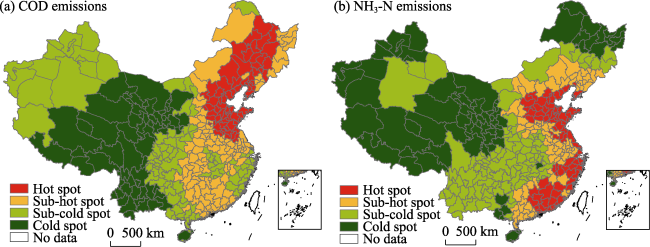
Figure 1 Hot-spot maps of COD and NH3-N emissions in China
The COD and NH3-N emissions are taken as the variables of central units, and the economic agglomeration is used as the variable of surrounding units to calculate the global bivariate Moran’s I. As shown in Table 4, the bivariate Moran’s I of the economic agglomeration and NH3-N emissions are 0.2025 and 0.2737, respectively, both of which pass the significance test ate 1% level. This indicates that there is a significant difference in the degree of spatial correlation between economic agglomeration and water pollutant emissions; that is, the higher the level of economic agglomeration, the more prominent the water pollutant emissions. In addition, the Moran’s I index of economic agglomeration and NH3-N emissions is larger than that of COD emissions, which means that the high-intensity NH3-N emissions tend to be distributed in cities with a higher economic agglomeration level. A comparative analysis of the bivariate Moran’s I index of economic level and pollutant emissions shows that the economic agglomeration has a greater spillover effect on water pollutant emissions than does the economic development level.
Table 4 Moran’s I of univariate and bivariate spatial correlations for water pollutant emissions
Pollutant
emissions
Univariate
analysis
Bivariate analysis
With economic agglomeration With economic level
COD Moran’s I 0.2575 0.2025 0.1469
P value 0.0010 0.0100 0.0010
NH3-N Moran’s I 0.2542 0.2737 0.1188
P value 0.0010 0.0100 0.0030

4.2 Analysis of local spatial autocorrelation

Based on the z-test (P = 0.05), bivariate LISA cluster maps are formed to identify the main spatial correlation pattern of economic agglomeration and water pollutant emissions (Figure 2), including high agglomeration-high emissions (High-High), high agglomeration-low emissions (High-Low), low agglomeration-high emissions (Low-High), low agglomeration-low emissions (Low-Low). Additionally, the bivariate LISA cluster maps also include a random pattern with no significant spatial correlation (Not sig.).
Figure 2 Bivariate LISA cluster maps of water pollutant emissions
(1) High-High regions. Both the levels of economic agglomeration and the water pollutant emissions are relatively high in these regions. The regions with high economic agglomeration and high COD emissions, including 24 cities across the country, are mainly distributed in northern and northeastern China, emanating from the Harbin-Changchun urban agglomeration and Beijing-Tianjin-Hebei region to the Shandong Peninsula. The regions of high economic agglomeration and high NH3-N emissions are distributed in Beijing, Tianjin, southwestern Shandong, central and northern Jiangsu, Fujian, and the Pearl River Delta urban agglomeration, including 28 cities. In these regions, the levels of economic agglomeration and industry density are particularly high, and large-scale economic agglomeration accelerates pollutant emissions. Among them, Beijing, Tianjin, Xuzhou, Zaozhuang, Jining, Rizhao, Linyi, and Yiyang are classified as High-High regions in terms of two kinds of water pollutant emissions at the city level. It can be seen that in order to alleviate regional water pollution in Beijing, Hebei, and southwestern Shandong, it is very important to control the scale of economic agglomeration and accelerate the formation of an environmentally friendly industrial structure.
(2) High-Low regions. The number of cities in this group is relatively small. Specifically, the regions of high economic agglomeration and low COD emissions mainly include Lüliang, Panzhihua, Liangshan, and Qujing. The regions of high economic agglomeration and low NH3-N emissions consist of Baotou, Erdos, Yulin, Panzhihua, Liangshan, and Nanning. Compared with the High-High regions, the water environmental pollution in this group is not very severe, but with a further increase in industrial agglomeration, these may be the regions where the water pollutant emission will increase rapidly in the future.
(3) Low-High regions. In these regions, the level of economic agglomeration is relatively low, but the water pollutant emissions are relatively high. The regions with low economic agglomeration and high COD emissions, including 14 cities, are mainly distributed around the high agglomeration-high emissions regions in northeastern and northern China. The regions with low economic agglomeration and high NH3-N emissions include Lianyungang, Jingzhou, Xianning, Shaoyang, Shaoguan, Huizhou, Hengshui, Kaifeng, and Xinyang. Although the level of economic agglomeration of these cities is relatively low, due to the high proportion of agricultural production involving livestock and poultry breeding, and aquaculture and crop production, the pollutant emissions of the cities, due to the agricultural sources, are quite large. The average proportions of agricultural COD and NH3-N emissions in Low-High regions are 68.15% and 40.04%, respectively, which are significantly higher than those in other types of cities. It can be seen that agricultural nonpoint source pollution should be mitigated through green prevention and control in these regions, including improving the efficiency of agricultural water use and reducing the use of pesticides and fertilizers. In addition, water pollutant emissions are increasing faster due to the spillover effects of adjacent high-emission cities.
(4) Low-Low regions. In these regions, both the levels of economic agglomeration and the water pollutant emissions are relatively low. These regions are widely distributed and concentrated in the Qinghai-Tibet Plateau and its marginal areas, including provincial-level areas of Tibet, Qinghai, Xinjiang, Gansu and Ningxia, and the cities in western Inner Mongolia, northwestern Yunnan, and western Sichuan. Most of these cities are located in the northwest of the “Hu Huanyong Population Line”, where the population is sparse and the economic density relatively low. Large-scale undeveloped resources and spaces and traditional agricultural production and living patterns result in relatively low levels of water pollutant emissions. The average COD and NH3-N emissions are 23,500 tons and 2200 tons, respectively, which are only 1/5 and 1/6 the average emissions of High-High regions. Generally, this group should control the emissions from urban residents and industries in the future.

5 Conclusions and policy implications

Based on the COD and NH3-N emissions Database of 339 Cities at city level in China, this study explores the impact of economic agglomeration on water pollutant emissions and the differences in magnitude of the impact on different-sized cities. The study also analyzes the spillover effect of economic agglomeration on water pollutant emissions. The results show that economic agglomeration can effectively reduce water pollutant emissions and is negative in all estimates of the whole, coastal, and inland samples. For the whole sample, a 1% increase in economic agglomeration reduces COD emissions and NH3-N emissions by 0.117% and 0.102%, respectively. These findings indicate that as economic activity increases the external spillover effects of capital investment, production technology, and emission reduction processes become more pronounced, increasing the efficient regional use of resources and energy and promoting the improvement of regional water environments. In addition, water pollutant emissions are mainly driven by factors such as industrialization and population growth and urbanization, reflecting that the current coupling pattern of industrialization and high emissions does not change. Both population growth and rapid urbanization accelerate water pollutant emissions.
Compared with large and megacities, economic agglomeration have a more prominent effect on the emission reduction of water pollution in small- and medium-sized cities. With a substantial increase in city size, the negative externalities of economic agglomeration and population expansion become cumulatively enlarged, resulting in an increase in the environmental load of the industrial layout. In other words, economic agglomeration plays a significant role in decreasing COD emissions in small- and medium-sized cities, indicating that solving water pollution problems in these types of areas is key to reducing emission intensity in the processes of urbanization. Therefore, differentiated policies should be formulated to guide industrial agglomeration and diffusion in the process of industrialization and urbanization. On the one hand, small- and medium-sized cities should be actively developed, and the emission reduction effect of economic agglomeration should be further enforced. The government should spatially promote moderate agglomeration of economic activity to achieve economies of scale and produce technology spillover effects. On the other hand, it is necessary to reasonably control the pollution-intensive industry scale and population scale of large and megacities, and to accelerate the adjustment of industrial structures to eliminate backward production capacity, which has high energy consumption and high pollution output. Additionally, the threshold for environmental access and control of the total amount of pollutant emissions must be raised substantially.
There is a significant spatial correlation between economic agglomeration and water pollutant emissions. The bivariate Moran’s I index of economic agglomeration and COD emissions (or NH3-N emissions) is 0.2025 (or 0.2737). Regions with high-intensity emissions tend to be distributed in areas with higher levels of economic agglomeration. The bivariate LISA cluster map shows that the spatial spillover effect of economic agglomeration and water pollutant emissions is significant, and it is characterized by four spatial correlation modes: high agglomeration-high emissions, low agglomeration-low emissions, low agglomeration-high emissions, and high agglomeration-low emissions. The high agglomeration-high emissions regions are mainly distributed in Beijing-Tianjin-Hebei region, and the Harbin- Changchun urban agglomeration. Among them, Beijing, Tianjin, and southwestern Shandong are both high agglomeration-high emissions regions with two kinds of water pollutant emission. Low agglomeration-low emissions regions are mainly distributed in the Qinghai-Tibet Plateau and its marginal areas. Low agglomeration-high emissions regions are mainly distributed in the periphery of the high agglomeration-high emissions regions in northeastern and northern China. In the future, it will be necessary to strengthen environmental protection and governance cooperation across administrative regions by focusing on the joint prevention and control of high agglomeration-high emissions regions and low agglomeration-high emissions regions. For different water pollutant emissions, a multi-scale coupled water environment integrated control unit, where watersheds and administrative districts are nested within each other, should be formed to minimize the spatial spillover effects of economic agglomeration and water environmental pollution.
Overall, this study is conducive to a firmer understanding of the relationship between economic agglomeration and water pollutant emissions. However, there are still some areas that require further research: (1) exploring in depth the different critical thresholds of economic agglomeration affecting water pollutant emissions; (2) revealing the feedback mechanism of water pollutant emissions on economic agglomeration; (3) further analyzing the environmental properties and conjugation effects of various water pollutants, which can provide a reference for determining the factors’ weights and integrating them into water-environment capacity assessments.
1
Chen D, Chen S, Jin H , 2018a. Industrial agglomeration and CO2 emissions: Evidence from 187 Chinese prefecture-level cities over 2005-2013. Journal of Cleaner Production, 172:993-1003.

DOI

2
Chen M, Liu W, Lu D et al., 2018b. Progress of China’s new-type urbanization construction since 2014: A preliminary assessment. Cities, 78:180-193.

DOI

3
Cheng Z , 2016. The spatial correlation and interaction between manufacturing agglomeration and environmental pollution. Ecological Indicators, 61:1024-1032.

DOI

4
Churchill S, Inekwe J, Ivanovski K et al., 2018. The Environmental Kuznets Curve in the OECD: 1870-2014. Energy Economics, 75:389-399.

DOI

5
Ciccone A, Hall R E , 1996. Productivity and the density of economic activity. The American Economic Review, 86(1):54-70.

DOI PMID

6
Ellison G, Glaeser E L , 1999. The geographic concentration of industry: Does natural advantage explain agglomeration? American Economic Review, 89(2):311-316.

DOI

7
Fang C, Zhou C, Gu C et al., 2017. A proposal for the theoretical analysis of the interactive coupled effects between urbanization and the eco-environment in mega-urban agglomerations. Journal of Geographical Sciences, 27(12):1431-1449.

DOI

8
Ferard J F, Blaise C , 2013. Encyclopedia of Aquatic Ecotoxicology. Dordrecht: Springer Science.

DOI PMID

9
Frank A, Moussiopoulosb N, Bartonovac A et al., 2001. Urban air quality in larger conurbations in the European Union. Environmental Modelling & Software, 16(4):399-414.

DOI PMID

10
Grossman G, Kuerger A , 1995. Economic, growth and the environment. Quarterly Journal of Economics, 110(2):353-377.

DOI PMID

11
Guo J, Xu Y, Pu Z , 2016. Urbanization and its effects on industrial pollutant emissions: An empirical study of a Chinese case with the spatial panel model. Sustainability, 8(8):812.

DOI

12
Han F, Xie R, Fang J et al., 2018. The effects of urban agglomeration economies on carbon emissions: Evidence from Chinese cities. Journal of Cleaner Production, 172:1096-1110.

DOI

13
Hao Y, Wu Y, Wang L et al., 2018. Re-examine Environmental Kuznets Curve in China: Spatial estimations using environmental quality index. Sustainable Cities and Society, 42:498-511.

DOI

14
Hosoe M, Naito T , 2006. Trans-boundary pollution transmission and regional agglomeration effects. Papers in Regional Science, 85(1):99-120.

DOI

15
Hossein H M, Kaneko S , 2013. Can environment quality spread through institutions? Energy Policy, 56(2):312-321.

DOI PMID

16
Hu Y, Cheng H , 2013. Water pollution during China’s industrial transition. Environmental Development, 8:57-73.

DOI

17
Ji X, Zhang W, Jiang M et al., 2017. Black-odor water analysis and heavy metal distribution of Yitong River in Northeast China. Water Science and Technology, 76(8):2051-2064.

DOI PMID

18
Li J, Chen Y, Li Z et al., 2018. Quantitative analysis of the impact factors of conventional energy carbon emissions in Kazakhstan based on LMDI decomposition and STIRPAT model. Journal of Geographical Sciences, 28(7):1001-1019.

DOI

19
Li Y, Luo E, Zhang H et al., 2018. Measuring interregional spillover and feedback effects of economy and CO2 emissions: A case study of the capital city agglomeration in China. Resources, Conservation and Recycling, 139:104-113.

DOI

20
Liang W, Yang M , 2019. Urbanization, economic growth and environmental pollution: Evidence from China. Sustainable Computing: Informatics and Systems, 21:1-9.

DOI PMID

21
Liu D, Xiao B , 2018. Can China achieve its carbon emission peaking? A scenario analysis based on STIRPAT and system dynamics model. Ecological Indicators, 93:647-657.

DOI PMID

22
Liu G Y, Yang Z F, Tang Y C et al., 2017a. Spatial correlation model of economy-energy-pollution interactions: The role of river water as a link between production sites and urban areas. Renewable & Sustainable Energy Reviews, 69:1018-1028.

DOI PMID

23
Liu S, Zhu Y, Du K , 2017b. The impact of industrial agglomeration on industrial pollutant emission: Evidence from China under New Normal. Clean Technologies and Environmental Policy, 19(9):2327-2334.

DOI

24
Liu Y, Zhou Y, Wu W ., 2015. Assessing the impact of population, income and technology on energy consumption and industrial pollutant emissions in China. Applied Energy, 155:904-917.

DOI

25
Lu Dadao , 2015. Moderate-speed growth: Sustainable development of China’s economy. Scientia Geographica Sinica, 35(10):1207-1219. (in Chinese)

26
Qi Wei, Liu Shenghe, Jin Haoran , 2016. Applicability of the new standard of city-size classification in China. Progress in Geography, 35(1):47-56. (in Chinese)

DOI

27
Scholten M C T, Foekema E M, Dokkum H P V et al., 2005. Eutrophication Management and Ecotoxicology. Berlin: Springer Berlin Heidelberg.

DOI PMID

28
Su W, Liu Y, Wang S et al., 2018. Regional inequality, spatial spillover effects, and the factors influencing city-level energy-related carbon emissions in China. Journal of Geographical Sciences, 28(4):495-513.

DOI

29
Thisse J F , 2018. Human capital and agglomeration economies in urban development. The Developing Economies, 56(2):117-139.

DOI PMID

30
Ushifusa Y , 2013. Productivity and labor density: Agglomeration effects over time. Atlantic Economic Journal, 41(2):123-132.

DOI

31
Verhoef E T, Nijkamp P , 2002. Externalities in urban sustainability: Environmental versus localization-type agglomeration externalities in a general spatial equilibrium model of a single-sector monocentric industrial city. Ecological Economics, 40(2):157-179.

DOI

32
Wang C, Wang F, Zhang X et al., 2017. Examining the driving factors of energy related carbon emissions using the extended STIRPAT model based on IPAT identity in Xinjiang. Renewable and Sustainable Energy Reviews, 67:51-61.

DOI

33
Wang J, Ye X, Wei Y D , 2019. Effects of agglomeration, environmental regulations, and technology on pollutant emissions in China: Integrating spatial, social, and economic network analyses. Sustainability, 11(2):363.

DOI

34
Wang Xiaoshuo, Yu Chaoyi , 2017. Impact of spatial agglomeration on industrial pollution emissions intensity in China. China Environmental Science, 37(4):1562-1570. (in Chinese)

PMID

35
Wang Z, Jia H F, Xu T et al., 2018. Manufacturing industrial structure and pollutant emission: An empirical study of China. Journal of Cleaner Production, 197(1):462-471.

DOI PMID

36
Xu B, Lin B , 2016. Regional differences of pollution emissions in China: Contributing factors and mitigation strategies. Journal of Cleaner Production, 112:1454-1463.

DOI

37
York R, Rosa E A, Dietz T , 2003. STIRPAT, IPAT and ImPACT: Analytic tools for unpacking the driving forces of environmental impacts. Ecological Economics, 46:351-365.

DOI

38
Yu Shuyi, Gao Feng, Zhang Yan , 2013. Economic growth, investment structure and environmental effect: Empirical study on the three economic regions in China. East China Economic Management, 27(6):70-77. (in Chinese)

39
Zhang C, Wang Y, Song X et al., 2017. An integrated specification for the nexus of water pollution and economic growth in China: Panel cointegration, long-run causality and Environmental Kuznets Curve. Science of the Total Environment, 609:319-328.

DOI PMID

40
Zhang Cuiju, Zhang Zongyi , 2016. Effect of spatial agglomeration of industry and population on China’s regional carbon emission intensity. Technology Economics, 35(1):71-77, 125. (in Chinese)

41
Zhang Xubo, Yu Wei, Zhang Yali et al., 2018. Spatial and temporal variation and influencing factors of economic growth in Beijing-Tianjin-Hebei region. Acta Geographica Sinica, 73(10):1985-2000. (in Chinese)

DOI

42
Zhao X F, Deng C L, Huang X J et al., 2017. Driving forces and the spatial patterns of industrial sulfur dioxide discharge in China. Science of the Total Environment, 577:279-288.

DOI PMID

43
Zhao Y M , 2017. The situation and countermeasures of soil and water pollution prevention and control in China. The People’s Congress of China, ( 9):46-51.

44
Zhou L, Zhou C, Yang F et al., 2019. Spatio-temporal evolution and the influencing factors of PM2.5 in China between 2000 and 2015. Journal of Geographical Sciences, 29(2):253-270.

DOI

Outlines

/