Research Articles

Does geographic distance have a significant impact on enterprise financing costs?

  • SUN Wei 1, 2 ,
  • LI Qihang 3 ,
  • LI Bo , 1, 4
Expand
  • 1. Institute of Geographic Sciences and Natural Resources Research, CAS, Beijing 100101, China
  • 1. College of Resources and Environment, UCAS, Beijing 100049, China
  • 1. Shandong University of Finance and Economics, Jinan 250014, China
  • 1. International College of Business and Technology, Tianjin University of Technology, Tianjin 300384, China
Li Bo (1981–), Associate Professor, E-mail:

Sun Wei (1975─), Associate Professor, specialized in regional development and spatial planning. E-mail: sunw@igsnrr.ac.cn

Received date: 2019-05-30

  Accepted date: 2019-07-29

  Online published: 2019-12-06

Supported by

Strategic Priority Research Program of the Chinese Academy of Sciences, No(XDA19040401)

Youth Fund for Humanities and Social Sciences of the Ministry of Education of China, No(16YJCZH040)

Youth Fund for Humanities and Social Sciences of the Ministry of Education of China, No(14YJCZH078)

National Natural Science Foundation of China, No(41571117)

National Natural Science Foundation of China, No(41871117)

Social Science Foundation of Beijing, No(14CSB010)

Shandong Taishan Scholar Youth Expert Support Program

Copyright

Copyright reserved © 2019. Office of Journal of Geographical Sciences All articles published represent the opinions of the authors, and do not reflect the official policy of the Chinese Medical Association or the Editorial Board, unless this is clearly specified.

Abstract

As information technology has been applied more broadly and transportation infrastructure has improved, persistent debate has existed as to the question of whether geographic distance influences enterprise financing costs (EFCs). Through mining big data regarding industrial enterprises and commercial bank branches (CBBs) in the Beijing-Tianjin-Hebei region, this paper conducts quantitative analysis of correlation between the EFCs and their distance to CBBs as well as the number of CBBs within a 1-5 km radius, and investigates how geographic factors affect EFCs. The results indicate the following: (1) In overall terms, the shorter the distance to CBBs and the greater the number of CBBs within a 1-5 km radius, the lower the EFCs. (2) Distance to CBBs and number of CBBs within a 1-5 km radius significantly influence state-owned and non-state-owned enterprises, with the effect on non-state-owned enterprises being more pronounced. (3) The EFCs in Beijing and Tianjin are not correlated with distance to CBBs, and negatively correlated to the number of CBBs within a 1-5 km radius; the EFCs in Hebei Province are positively correlated with distance to CBBs, and negatively correlated with the number of CBBs within a 1-5 km radius. (4) Distance to CBBs has a more significant impact on enterprises engaged in heavy industry and labor-intensive industries, while there is not much difference between different industries in terms of how the number of CBBs within a 1-5 km radius affects them.

Cite this article

SUN Wei , LI Qihang , LI Bo . Does geographic distance have a significant impact on enterprise financing costs?[J]. Journal of Geographical Sciences, 2019 , 29(12) : 1965 -1980 . DOI: 10.1007/s11442-019-1699-6

1 Introduction

Financing is an important factor in enterprise growth. It is difficult for enterprises to meet all of their financing needs by relying solely on internally accumulated funds, and therefore they must opt for external financing when internal funds cannot meet their needs (Lu and Qiu, 2016). The 2008 international financial crisis hit the global economy hard, causing a long-term downturn that will make the global economy grow more slowly over the next 10-20 years than it did over the last 20 years. Feeling the impact of a drop in effective demand both internationally and domestically, China’s real economy is facing numerous challenges to its growth, one of which is the difficulty and high costs of securing financing. In order to spur growth of the real economy, the government has implemented a series of financial and fiscal policies to support enterprise growth, which focus on the key issues of developing primary-level operations networks and cutting financing costs. In 2015, the China Banking Regulatory Commission released a publication stressing the need to boost the development of CBBs and expand network coverage to truly reduce EFCs. But will expanding the coverage of the network of CBBs help cut EFCs? In other words, do the number of CBBs and the distance of these branches to enterprises have a substantial effect on financing costs?
Whether or not geographic distance affects EFCs has been a subject of continuous debate among scholars. Some believe that the relative impact of geographic factors on financial institutions’ choice of location has decreased along with the widespread application of information technology and improvement of transportation infrastructure. For example, Petersen et al. (2002) showed that increased financing for small-sized enterprises does not result from geographic factors such as greater proximity to banks or clustering of financial institutions, but is instead owed to the rising productivity of banks, while Degryse et al. (2005) and Carling et al. (2005) used loan data from certain large banks in Belgium and Sweden, respectively, to examine the impact of geographic distance between banks and enterprises on interest rates, finding that there was no significant impact. Despite this, the majority of researchers argue that we should not simply infer that the impact of geographic distance on EFCs has already faded away. For example, Porteous (1995) argued that geographic distance between creditors and debtors is still an important factor affecting financial transactions. In the non-standardized financial products market, information asymmetry amplifies spatial effects, so closeness between a bank and a borrower in terms of distance and relationship reduces risks related to non-standardized loans. Brevoort et al. (2006) used small and medium-sized enterprise data to examine the impact of distance between banks and enterprises on business loans, finding that distance indeed impedes the number of loans from rising and has a greater effect on small banks than large banks. Robert et al. (2006) established a model centered on the relationship between informational distance and banks’ investment in information technology, with their research indicating that as competition intensifies, banks tend to grant loans to nearby enterprises. Turner (2011) pointed out that financial frictions are inherently spatially varied, with this type of variation showing that geographic differences can have a relatively large effect on financial transactions. For example, geographic factors frequently become difficult obstacles when banks attempt to establish or maintain a relationship with a client. Knyazeva et al. (2012) put forward new evidence on the function of distance in the creditor-debtor relationships between banks and borrowers, finding that the difficultly of obtaining and verifying soft information from enterprises beyond a certain distance can result in relatively high information collection costs, which in turn leads to distance-related information collection and monitoring expenses being reflected on various levels such as loan methods, spreads, collateral, and contracts.
In sum, studies on enterprise financing are primarily concentrated in the fields of finance and economics. Although very few geographers have entered into this field of study, interest in the field has consistently increased in recent years. Due to differences and limitations in terms of research perspectives and methods, research on this topic focuses more on the financial factors of enterprises themselves, such as the nature and scale of enterprises and fixed or collateralizable assets, as well as other elements in the financial ecosystem such as government support and credit guarantee systems. There are very few studies that employ an approach such as the distance between enterprises and CBBs and the number of branches within a certain radius from enterprises to conduct empirical research on this topic. Though certain studies have noted geography-related issues such as the geographic distance and proximity between banks and enterprises, they have not attached enough importance to these issues. Therefore, this study uses ordinary least squares (OLS) regression and the Tobit model to conduct quantitative analysis of the correlation between the financing costs of industrial enterprises in the Beijing-Tianjin-Hebei region and the two factors of the distance of these enterprises to CBBs and the number of branches within a certain radius by mining big data regarding CBBs and industrial enterprises, and examines the mechanisms by which these two geographic factors influence EFCs. It therefore offers scientific reference for the government’s formulation and adjustment of relevant fiscal and financial policies, particularly those that promote increasing the number of CBBs and improving network coverage in a reasonable manner, as well as for driving forward coordinated development in the Beijing-Tianjin- Hebei region.

2 Methods and data sources

2.1 Methods

Looking at existing research and the experience of economic development in China, it can be seen that a clear link exists between the EFCs and their geographic distance to CBBs. Turner (2011) pointed out that geographic differences bring challenges to financial relationships. For banks to build and maintain relationships with clients, there are certain geographic barriers that are difficult to overcome, setting aside the challenge of each region having its own unique industries and business networks with independent cultures. Geographic distance brings not only transportation costs, but also information asymmetry, which in turn impacts EFCs. According to this inference and information asymmetry theory in economics, the information asymmetry generated by geographic distance will form growing mutual distrust between borrowers and lenders, which will then lead to adverse selection and moral hazard. The two effects described above will both constantly raise interest rates and reduce the number of loans, ultimately shrinking the market for loans or, in extreme circumstances, causing lenders to withdraw from certain areas. In practice, commercial banks widely employ auditing methods that favor practicality over financial statements, and participate in the supervision and management of enterprises in certain ways. A geographic advantage is beneficial when banks are deciding whether or not they would like to engage in long-term interaction and mutual supervision as well as determining the breadth and depth of their involvement, because it guarantees the security and profitability of their capital. In view of the above, we put forward the following hypothesis (hypothesis 1) from the geographic perspective: where other conditions are constant, enterprises will have lower financing costs the closer they are to CBBs.
According to the findings of Hernández et al. (2010) as the monopoly of banks over the market becomes stronger, borrows have less flexibility in procuring a loan and business loan costs increase. Kysucky et al. (2016) pointed out that the level of competition between banks is the key factor determining how loan costs are split between borrowers and lenders. There are certain limitations on directly researching the level of competition within regions. In contrast to the scale of market monopolization for ordinary industries, the banking market has stronger geographic characteristics than pricing characteristics. This means the geographic radius of competition between banks is smaller. Therefore, attention should be paid to the level of competition within a geographic radius, especially when the research target is refined down to the branch level. There is currently limited geography-based research analyzing the impact of monopolization on financing costs. This paper thus puts forward the following hypothesis (hypothesis 2) from the geographic perspective: where other conditions are constant, enterprises will have lower financing costs the greater the number of CBBs within a certain radius.
The following research methods are employed to prove the two hypotheses. In line with the hypotheses, this study attempts to establish a regression model for EFCs and distance to CBBs / number of CBBs in the surrounding area:
$lfcost\_{{r}_{i}}\text{=}\alpha +{{\beta }_{1}}distanc{{e}_{i}}+{{\beta }_{2}}num\_{{b}_{i,k}}+\gamma \sum{{{g}_{j}}*X}+du{{m}_{city}}+du{{m}_{ind}}+{{\varepsilon }_{i}}$
where lfcost_r represents the EFCs; i indicates the enterprise; distance is the natural log of the mean distance of the three closest CBBs to the enterprise; num_b is the number of CBBs in the enterprise’s vicinity; k is the number of CBBs within a certain number of kilometers from the enterprise; a is the intercept; and εi is the normally distributed random error term. This paper controls for differences that could exist between some regions and industries by using region fixed effects (dumcity) and two-digit standard industrial classification (SIC2)-level industry fixed effects (dumind) dummy variables; X is the control variable vector; and β1, β2, and γ are coefficients. Other variables and their meanings are shown in Table 1.
Table 1 Definition and explanation of variables
Variable category Explanation
lfcost_r Natural logarithm of EFCs obtained by retaining positive values from dividing interest expenses by the difference between total liabilities and accounts payable, winsorized at top and bottom 1%
distance Natural logarithm of the mean distance to the three closest CBBs to the enterprise
num_1k Number of CBBs within a 1 km radius from the enterprise
num_3k Number of CBBs within a 3 km radius from the enterprise
num_5k Number of CBBs within a 5 km radius from the enterprise
lfa Natural logarithm of fixed assets
lwc Natural logarithm of operating capital
lworker Natural logarithm of number of employees
lev Leverage ratio (assets divided by liabilities)
dum_gov SOE dummy variable (has a value of 1 if state-owned shares account for more than 50% of paid-in capital, otherwise has a value of 0)
dum_for Foreign enterprise dummy variable (has a value of 1 if foreign capital shares (includes Hong Kong, Macao, and Taiwan) account for more than 25% of paid-in capital, otherwise has a value of 0)
dum_qg Light industry dummy variable (has a value of 1 if the industry fits in to the light category as defined by the national bureau of statistics, and a value of 0 if it fits into the heavy category)
dum_lab Labor intensive industry dummy variable (has a value of 1 if the ratio between number of workers and output value for industry as a whole is above the median of the same ratio for all industries, otherwise has a value of 0)

2.2 Data sources

The data used in this paper can be divided into two categories: enterprise data and CBB data.
Enterprise data comes from the 2013 China Industrial Enterprise Database, which includes all state-owned industrial enterprises as well as large non-state-owned enterprises. According to 2013 industry standards, large enterprises refers to enterprises with annual income of 20 million yuan or more from their main operations. Our calculations indicate that gross enterprise output included in the 2013 China Industrial Enterprise Database accounted for over 90% of gross industrial output in the Beijing-Tianjin-Hebei region. Industrial statistics indicators include the main economic and financial indicators such as liquid assets, financial expenses, and total profits, as well as region codes, names of administrative divisions, and exact addresses.
CBB data comes from information listed on the China Banking Regulatory Commission homepage up until May 1, 2015. It is possible to see online that there are a total of 12,424 CBBs in the Beijing-Tianjin-Hebei region. Using Stata, Excel, and other relevant tools, we manually matched each of the 12,424 CBBs with its corresponding prefecture-level city according to address information for the bank network in the raw data. For CBBs without a clearly indicated prefecture-level city, we matched them to their locations one-by-one by searching through relevant information, and completed their entries after confirming there were no errors. On the basis of the year that each CBB was established, which is recorded in the data, we collected exact addresses for every CBB in the Beijing-Tianjin-Hebei region in 2013 (Figure 1).
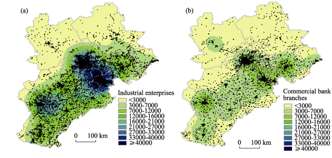
Figure 1 Kernel density estimation map for industrial enterprises (a) and banks (b) in the Beijing-Tianjin-Hebei region in 2013
In the process of sorting through outliers, we eliminated micro-enterprises (enterprises with less than eight employees), insolvent enterprises (enterprises with debt greater than the value of their assets), enterprises with excessively high interest rates (higher than 1), and enterprises missing interest rates. Meanwhile, in order to reduce the impact of extreme value errors, we processed outliers at the top and bottom 1% of continuous variables such as EFCs using winsorization (Nie et al., 2012).

2.3 Latitude and longitude coordinates and distance calculations

To reach the research goals of this paper, it was necessary to obtain the latitude and longitude coordinates of industrial enterprises and CBBs, and to calculate the distance between enterprises and CBBs. In line with the hypotheses, we attempted to calculate the following two measurement indexes: mean distance of the three closest CBBs to the enterprise, and number of CBBs within a 1-5 km radius.
Acquisition of coordinates. Latitude and longitude coordinates for CBBs and industrial enterprises are from the Baidu Maps Geocoding API. Using Python, we went through the addresses of each CBB and enterprise in order and entered them into the Geocoding API as parameters, and then saved the latitude and longitude coordinates that came back. As a result of network instability and the sheer volume of data, it is possible that some data was omitted. We therefore checked for omissions and filled in the gaps, and thus the missing data value was reduced to 2% or less.
Number of CBBs within a certain radius. While calculating distance to CBBs, we adopted the standard latitude and longitude distance method Via the R package of geographic distance, we calculated the spherical distance between each industrial enterprise and its three closest CBBs using the latitude and longitude coordinates of two points. Furthermore, we calculated the number of CBBs within circular coverage limits with enterprises at the center of the circles, drawing circles with radiuses of 1 km, 3 km, and 5 km based on the distance that can be travelled in 10 minutes on foot, riding a bicycle, or driving a car.

3 Analysis of results

First, we carried out Spearman correlation testing on each variable. Then, according to the distributional properties of the samples, we carried out regression analysis using the OLS and Tobit methods in order to verify whether or not geographic distance to CBBs or the number of CBBs within a certain radius have an effect on the EFCs. Lastly, we analyzed the differences in these effects between different enterprises, industries, and regions.

3.1 Correlation testing and estimation method selection

According to our statistics, distance between industrial enterprises in the Beijing-Tianjin-Hebei region and their three closest CBBs had a logarithmic mean value of 8.07, a minimum value of 0, and a maximum value of 14.09. The mean value for the number of CBBs was 2.33 within a 1 km radius, 11.92 within a 3 km radius, and 27.33 within a 5 km radius, but the median numbers were 1, 3, and 7 with maximum values of 51, 301, and 597, respectively. This indicates that CBBs are very unevenly distributed around industrial enterprises in the Beijing-Tianjin-Hebei region.
The results of Spearman correlation testing are shown in Table 2. The logarithm of EFCs is positively correlated with distance to CBBs, and negatively correlated with the number of CBBs within a certain radius. This shows that industrial enterprises have lower financing costs the closer they are to CBBs and the greater the number of CBBs within a certain radius around them. From correlation analysis of other variables, we found that apart from the numbers of CBBs within certain radiuses, between which there ought to be strong correlation (the numbers of CBBs within different radiuses were individually inputted into multiple regressions), none of the other variables had correlation coefficients over 0.5, while their variance inflation factors were all below 3.
Table 2 Correlation coefficients of variables
lfcost_r distance Num_1k Num_3k Num_5k lfa lev
distance 0.086*** 1
Num_1k -0.082*** -0.507*** 1
Num_3k -0.136*** -0.274*** 0.769*** 1
Num_5k -0.149*** -0.213*** 0.672*** 0.955*** 1
lfa 0.140*** -0.013 0.028*** 0.015* -0.003 1
lev -0.216*** -0.063*** 0.021*** 0.037*** 0.039*** -0.099*** 1

Note: The *, **, and *** symbols represent 10%, 5%, and 1% levels of significance, respectively

In order to control for excessive or unstable standard deviation, we needed to put the EFCs of industrial enterprises through logarithmic processing. As can be seen in Figure 2, a large amount of data on the EFCs logarithm scatterplot is concentrated around a value of zero, which does not satisfy the assumptions of OLS regression. After eliminating the zero value, however, the data has normal distribution. Therefore, when conducting OLS regression, samples with a value of zero must be eliminated for further analysis to be possible, while Tobit regression (censored at zero) should be carried out on all data for the purposes of comparison and robustness analysis.
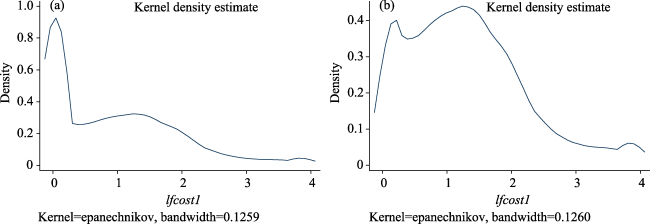
Figure 2 Kernel density estimation of financing cost logarithms with the full sample (a) and with zero values eliminated (b)

3.2 Regression analysis and hypothesis verification

Table 3 shows the results of OLS (whole sample) and Tobit regression analysis of EFCs with regard to other industrial enterprise data. The results indicate that the coefficients for distance to CBBs are positive and highly robust, which shows that being closer in distance to CBBs reduces EFCs. This proves hypothesis 1. The coefficients for number of CBBs within 1, 3, and 5 km radiuses are clearly negative, which shows that industrial enterprises have lower financing costs the greater the number of CBBs there are around them. This proves hypothesis 2.
Table 3 Results of OLS regression and Tobit regression of EFCs and other variables
Variables Regression (1) Regression (2) Regression (3) Regression (4) Regression (5) Regression (6)
OLS OLS OLS Tobit Tobit Tobit
distance 0.020** 0.018*** 0.019*** 0.022*** 0.019*** 0.021***
(2.69) (3.26) (3.32) (3.17) (3.07) (3.34)
num_1k -0.004 -0.005
(-1.17) (-1.31)
num_3k -0.002*** -0.003***
(-4.01) (-4.58)
num_5k -0.001*** -0.001***
(-3.69) (-5.08)
lfa 0.110*** 0.107*** 0.106*** 0.176*** 0.171*** 0.170***
(5.90) (5.73) (5.80) (13.54) (13.11) (13.01)
lwc -0.081 -0.076 -0.075 -0.055*** -0.047*** -0.046***
(-1.54) (-1.48) (-1.47) (-3.50) (-3.00) (-2.91)
lworker 0.009 0.012 0.013 0.004 0.008 0.009
(0.32) (0.42) (0.43) (0.19) (0.40) (0.43)
lev -1.034* -1.025* -1.024* -0.855*** -0.843*** -0.840***
(-2.00) (-2.00) (-2.00) (-12.34) (-12.16) (-12.13)
dum_gov 0.175* 0.182** 0.184** 0.287*** 0.299*** 0.301***
(2.08) (2.21) (2.22) (6.16) (6.40) (6.45)
dum_for -0.065 -0.069 -0.070 -0.084** -0.090** -0.092**
(-1.10) (-1.23) (-1.26) (-2.14) (-2.30) (-2.35)
City effects YES YES YES YES YES YES
Industry effects YES YES YES YES YES YES
City cluster-robust standard errors YES YES YES - - -
_cons 2.042** 2.014** 1.999** 0.938*** 0.902*** 0.879***
(2.97) (2.95) (2.94) (4.03) (3.89) (3.79)
N 11780 11780 11780 15987 15987 15987
Adjusted R2 0.225 0.226 0.226

Note: Numbers in brackets are the t values of regression coefficients. The *, **, and *** symbols represent 10%, 5%, and 1% significance levels, respectively.

There are two possible explanations for this. On the one hand, being closer allows CBBs to become directly involved in enterprises’ operations and production activities and gain a true understanding of their financial circumstances and growth prospects. Proximity makes it so that CBBs are not limited to relying on regular channels like financial statements to find out about enterprises and increases the sources and channels through which they can collect information, which makes this information more reliable. By implementing effective management over enterprises through informal channels, banks can steer clear of a series of information asymmetry problems brought through false financial statements, and to a large extent avoid moral hazard and financial losses. Meanwhile, as a result being closer in distance, enterprises will also cut down on deceptive practices by their own initiative in order to signal banks that they operate in an honest and trustworthy manner.On the other hand, the clustering of a relatively large number of CBBs in a specific location brings competitive effects and information sharing effects. Competitive effects mean that competition between CBBs puts the ball in the court of enterprises, since they can benefit from this type of competitive relationship by comparing details such as approval processes, loan amounts, and interest rates to choose the best credit product. Meanwhile, the beneficiaries of information sharing effects are CBBs. This is because the sharing of information between CBBs helps make enterprise information more transparent while also improving the quality of information supplied by enterprises, which allows CBBs to more effectively identify enterprises with different risks. Therefore competitive effects and information sharing effects can benefit both borrowers and lenders (industrial enterprises and CBBs), allowing them to achieve a “win-win.”In addition to the impact of the two factors described above on the EFCs, EFCs are also related to enterprises’ financial indicators. The fixed asset indicator (lfa) is markedly positive at the 1% level, which shows that enterprises have higher financing costs the larger the scale of their fixed assets as a result of liquidity issues. The owner’s equity index (lwc) is markedly negative at the 1% level, which shows that when an enterprise has quite a large amount of equity, its financing costs are relatively low. The leverage ratio index also illustrates this issue. EFCs are lower the higher their leverage ratio.

3.3 Differential analysis

3.3.1 Differences between regionsSince Beijing, Tianjin, and Hebei are very different in terms of the density with which financial institutions are distributed, they are also somewhat different in terms of the sensitivity of EFCs. We divided the region in two (Beijing-Tianjin and Hebei) and separated the results of regression on enterprises in each area in order to observe the differences between big cities and ordinary province (Table 4).Our findings show that the EFCs in Beijing and Tianjin are not related to distance to CBBs. To a certain extent, this shows that within the confines of urban space, distance is not one of the main influencing factors on EFCs. In terms of correlation with the number of CBBs within a certain radius, correlation was more significant within a 1 km radius in Beijing and Tianjin, and more significant within 3 km and 5 km radiuses in Hebei Province.3.3.2 Differences between industriesAccording to National Bureau of Statistics standards, we divided industries into the categories of light/heavy and labor-intensive/non-labor-intensive and carried out regression analysis in combination with both distance to CBBs and number of CBBs within a certain radius (Table 5).
Table 4 Results of OLS regression of EFCs (sample divided by provincial unit)
Variables Regression
(1)
Regression (2) Regression
(3)
Regression (4) Regression
(5)
Regression (6)
Beijing-Tianjin OLS Hebei OLS Beijing-Tianjin OLS Hebei OLS Beijing-Tianjin OLS Hebei OLS
distance 0.00537 0.0216 0.00526 0.0192** 0.00643 0.0213**
(2.188) (1.147) (1.903) (2.323) (3.250) (2.659)
num_1k -0.00535*** -0.00738
(-78.62) (-0.417)
num_3k -0.00149** -0.00462***
(-20.96) (-4.863)
num_5k -0.000590 -0.00225***
(-4.994) (-3.506)
lfa 0.0666* 0.0755** 0.0644* 0.0712** 0.0645* 0.0695**
(9.409) (2.634) (10.28) (2.531) (11.84) (2.539)
lwc -0.0867 -0.218*** -0.0835 -0.210*** -0.0836 -0.208***
(-1.801) (-9.332) (-1.770) (-9.123) (-1.810) (-9.167)
lworker -0.00807 0.0489 -0.00624 0.0563 -0.00594 0.0569
(-0.474) (1.156) (-0.389) (1.390) (-0.384) (1.428)
lev -0.828 -2.463*** -0.825 -2.433*** -0.825 -2.424***
(-3.177) (-13.02) (-3.244) (-13.17) (-3.243) (-13.47)
dum_gov -0.0590 -0.103 -0.0610 -0.102 -0.0623 -0.102
(-0.691) (-0.930) (-0.731) (-0.926) (-0.756) (-0.918)
City effects YES YES YES YES YES YES
Industry effects YES YES YES YES YES YES
City cluster-robust standard errors YES YES YES YES YES YES
_cons 2.358 4.775*** 2.350 4.699*** 2.328 4.663***
(2.087) (11.56) (2.053) (12.44) (2.039) (12.10)
N 3752 5533 3752 5533 3752 5533
Adjusted R2 0.073 0.206 0.0748 0.207 0.075 0.208

Note: Numbers in brackets are the t values of regression coefficients. The *, **, and *** symbols represent 10%, 5%, and 1% significance levels, respectively.

Our findings show that there is no correlation between distance to CBBs and the EFCs in the light industry category, but that there is notable correlation between the distance to CBBs and the EFCs in the heavy industry category. This could be related to the fact that for light industry, loan amounts are smaller and specialized information is limited. In essence, the influence of distance on EFCs should come from “soft information,” which includes personal interactions and evaluations of trustworthiness, as well as indications of social connections and operating conditions that are not reflected in financial statements. Meanwhile, the influence of distance on “hard information” such as financial information, collateral information, and standard endorsements is relatively weak. Furthermore, heavy industries borrow quite a lot of money, but due to the peculiarities of their trade and the fact that items of collateral backed by “hard information” (such as real estate) are often insufficient, the collateral that they put up most likely includes equipment. Equipment is different from real estate in that its liquidity depends on the true state of business operations, and this therefore causes CBBs to prefer working with enterprises that they know inside and out. Light and heavy industries both show marked correlation with regard to the number of CBBs within a certain radius, particularly within the 3 km and 5 km radiuses.
Table 5 Results of OLS regression of EFCs (sample divided according to the light and heavy industry categories)
Variables Regression (1) Regression (2) Regression (3) Regression (4) Regression (5) Regression (6)
Light industry OLS Heavy industry OLS Light industry OLS Heavy industry OLS Light industry OLS Heavy industry OLS
distance 0.0146 0.0224* 0.00781 0.0244** 0.00936 0.0260**
(1.134) (2.053) (1.135) (2.835) (1.344) (2.988)
num_1k 0.00157 -0.00819
(0.159) (-1.516)
num_3k -0.00268*** -0.00211***
(-5.250) (-3.742)
num_5k 0.00109*** -0.000850***
(-4.154) (-3.578)
lfa 0.0728** 0.0839*** 0.0677* 0.0815*** 0.0672* 0.0814***
(2.247) (5.488) (2.098) (5.628) (2.106) (5.739)
lwc -0.186*** -0.180*** -0.175*** -0.176*** -0.175*** -0.176***
(-3.660) (-5.151) (-3.530) (-5.143) (-3.625) (-5.178)
lworker 0.0368 0.0229 0.0415 0.0255 0.0410 0.0254
(1.186) (0.566) (1.313) (0.632) (1.298) (0.635)
lev -2.266*** -1.853*** -2.252*** -1.842*** -2.253*** -1.842***
(-5.049) (-5.830) (-5.084) (-5.869) (-5.114) (-5.872)
Dum_gov -0.0859 -0.0855 -0.0882 -0.0861 -0.0877 -0.0870
(-1.130) (-1.167) (-1.209) (-1.196) (-1.228) (-1.216)
City effects YES YES YES YES YES YES
Industry effects YES YES YES YES YES YES
City cluster-robust standard errors YES YES YES YES YES YES
_cons 4.283*** 4.052*** 4.270*** 3.998*** 4.262*** 3.982***
(8.526) (7.664) (8.215) (7.940) (8.325) (7.928)
N 2317 6968 2317 6968 2317 6968
Adjusted R2 0.268 0.181 0.269 0.182 0.269 0.182

Note: Numbers in brackets are the t values of regression coefficients. The *, **, and *** symbols represent 10%, 5%, and 1% significance levels, respectively.

Similarly, the EFCs in labor-intensive industries are more significantly correlated with distance to CBBs than those of enterprises in non-labor-intensive industries. This is, to a definite degree, due to the fact that the items which enterprises in labor-intensive industries use for collateral are relatively limited and belong more to the level of “soft information.” Labor-intensive and non-labor-intensive industries both show marked correlation with regard to the number of CBBs, particularly within the 3 km and 5 km radiuses (Table 6).
Table 6 Results of OLS regression of EFCs (sample divided according to labor-intensive industry and non-labor intensive industry categories)
Variables Regression (1) Regression
(2)
Regression (3) Regression
(4)
Regression (5) Regression
(6)
Intensive OLS Non-intensive OLS Intensive OLS Non-intensive OLS Intensive OLS Non-intensive OLS
distance 0.0235** 0.0155 0.0239*** 0.0152 0.0259*** 0.0163
(2.900) (1.337) (4.335) (1.550) (4.416) (1.666)
num_1k -0.00831 -0.00389
(-1.509) (-0.781)
num_3k -0.00275*** -0.00162**
(-4.603) (-2.808)
num_5k -0.00107*** -0.000660**
(-3.733) (-2.778)
lfa 0.0712** 0.0876*** 0.0674** 0.0850*** 0.0671** 0.0850***
(2.625) (3.570) (2.508) (3.556) (2.522) (3.588)
lwc -0.177*** -0.181*** -0.170*** -0.177*** -0.171*** -0.177***
(-4.226) (-5.142) (-4.144) (-5.133) (-4.205) (-5.197)
lworker 0.0312 0.0162 0.0343 0.0188 0.0339 0.0188
(0.875) (0.496) (0.952) (0.583) (0.953) (0.587)
lev -2.106*** -1.838*** -2.091*** -1.830*** -2.091*** -1.829***
(-5.469) (-5.420) (-5.501) (-5.458) (-5.515) (-5.470)
Dum_gov -0.105 -0.0680 -0.105 -0.0699 -0.106 -0.0700
(-1.533) (-0.981) (-1.562) (-1.033) (-1.607) (-1.039)
City effects YES YES YES YES YES YES
Industry effects YES YES YES YES YES YES
City cluster-robust standard errors YES YES YES YES YES YES
_cons 3.128*** 3.965*** 3.078*** 3.937*** 3.066*** 3.925***
(4.747) (7.532) (4.770) (7.686) (4.754) (7.681)
N 4201 5084 4201 5084 4201 5084
Adjusted R2 0.226 0.197 0.228 0.198 0.228 0.198

Note: Numbers in brackets are the t values of regression coefficients. The *, **, and *** symbols represent 10%, 5%, and 1% significance levels, respectively.

3.4 Endogeneity analysis

Endogeneity is an issue that all studies must pay attention to. Even though the geographic distance factor used in this paper is not significantly affected by the characteristics of individual enterprises, a certain amount of endogeneity still exists. This comes from the possible existence of omitted variables, as well as the problem of simultaneity (mutual causation) brought about by the two-way self-selection of CBBs and enterprises. Therefore, in the regression carried out above, we used the dummy variables of which industries and prefecture-level cities enterprises belong to in order to control for potentially omitted industry and region variables.
However, it is irrefutable that endogeneity still exists with regard to EFCs and the distance between CBBs and enterprises on the micro level. For this reason, we obtained the mean and variance for the topographic gradients of all prefecture-level cities, which we used as instrumental variables. Theoretically speaking, if a prefecture-level city has a relatively large gradient, then objectively its population and enterprises will be more concentrated in flat areas, which will have a corresponding impact on the distance between enterprises and CBBs. However, this geographic pattern will not directly influence EFCs, thus controlling for endogeneity (Table 7).
Table 7 Results of OLS and IV-2SLS regression of EFCs
Variables Regression (1) Regression (2) Regression (3) Regression (4)
OLS IV IV IV
ldis 0.074*** 0.698*** 0.374** 0.377**
(6.67) (3.78) (2.56) (2.36)
lfa 0.105*** 0.069*** 0.071***
(9.57) (2.65) (2.94)
lwc -0.091** -0.038 -0.027
(-2.30) (-0.83) (-0.64)
lworker 0.039 0.076* 0.055*
(1.43) (1.74) (1.75)
lev -0.951** -0.837*** -0.755***
(-2.95) (-2.93) (-3.05)
dum_gov 0.438*** 0.435*** 0.389***
(6.77) (4.46) (4.59)
dum_for -0.019 -0.044 -0.049**
(-0.43) (-1.64) (-2.18)
_cons 0.828 -4.352*** -2.343* -2.043
(1.50) (-3.33) (-1.84) (-1.45)
IV No Yes Yes Yes
Fixed effects Yes No No Yes
Cluster-robust Yes Yes Yes Yes
N 14845 14845 14845 14845
Adjusted R2 0.243 -0.383 0.093 0.132
Weak instruments test 12.343 8.135 9.799
Overidentification test 3.260 3.691 5.361
0.196 0.158 0.069
Endogeneity test 5.653 3.183 1.753
0.019 0.078 0.215

Note: Numbers in brackets are the t values of regression coefficients. The *, **, and *** symbols represent 10%, 5%, and 1% significance levels, respectively.

In Table 7, the first column shows the results of OLS regression for comparison, while columns 2-4 show the estimated results of IV two-stage least squares (2SLS) regression. The results show that after gradually adding control variables and fixed effects, geographic distance maintains a significant positive impact on the EFCs. The results of weak instrumental variable (Cragg-Donald or Kleibergen-Paap) test and first-stage regression (not listed due to space limitations) all indicate that the instrumental variables used in this paper are significant. The overidentification test (Anderson-Rubin overidentification LR statistic) indicates that the results of regression cannot reject the original hypotheses at a 5% level of significance, which shows that overidentification does not exist. The result of Anderson-Rubin F-test of significance of endogenous regressors is significant before controlling for fixed effects, which indicates that instrumental variables serve a purpose since there is significant difference between results obtained using instrumental variables and those obtained without using instrumental variables. This outcome gradually becomes less significant as control variables and fixed effects are added, which shows that the majority of endogeneity comes from omitted variables rather than self-selection.

4 Conclusions and discussion

4.1 Conclusions

This paper used OLS regression and the Tobit models to conduct quantitative analysis of how the EFCs within the Beijing-Tianjin-Hebei region are correlated with distance to CBBs and the number of CBBs within a certain radius. The results of the study are as follows:
(1) The EFCs are not only influenced by factors such as scale of fixed assets, owner’s equity, and leverage ratio, they are also affected by the geographic distance to CBBs and the number of CBBs within a certain radius. EFCs will be lower the closer it is to CBBs and the more CBBs there are within a certain radius.
(2) Geographic factors produce effects through two main mechanisms. On the one hand, being closer in proximity broadens the channels through which CBBs can collect information. This allows them to get a realistic understanding of how enterprises are running and avoid problems of information asymmetry brought about by false financial statements. On the other hand, the clustering of CBBs in a particular location brings competitive effects and information sharing effects.
(3) Distance to CBBs significantly affects the EFCs of both state-owned enterprises and non-state-owned enterprises. Comparatively speaking, the effect on non-state-owned enterprises is more pronounced. In terms of correlation with the number of CBBs within a certain radius, non-state-owned enterprises show stronger correlation than state-owned enterprises. In addition, correlation is more significant for both state-owned and non-state-owned enterprises within the 3 km and 5 km radiuses than within the 1 km radius.
(4) Differences exist between regions in terms of sensitivity to distance. The EFCs in Beijing and Tianjin are not correlated with distance to CBBs, while those of enterprises in Hebei Province are positively correlated with the latter. To a certain extent, this shows that within the confines of urban space, distance is not one of the main influencing factors on EFCs. In terms of correlation with the number of CBBs within a certain radius, Beijing and Tianjin show more significant correlation within the 1 km radius, while Hebei Province shows more significant correlation within the 3 km and 5 km radiuses.
(5) Differences also exist between industries in terms of sensitivity to distance. The EFCs in light industry are not correlated with distance to CBBs, while the relationship between heavy industries and distance to CBBs is more significant. Meanwhile, the EFCs in labor-intensive industries are more significantly correlated with distance to CBBs than those of enterprises in non-labor-intensive industries. This is, to a definite degree, due to the fact that the items which enterprises in labor-intensive industries use for collateral are relatively limited and belong more to the level of “soft information.” There is quite significant correlation between the number of CBBs within a certain radius and the EFCs in both light and heavy industry and both labor-intensive and non-labor-intensive industries, particularly within the 3 km and 5 km radiuses.
Through our analysis of the influencing factors on the EFCs in the Beijing-Tianjin-Hebei region, we reached the important realization that expanding the coverage of CBBs is conducive to reducing the EFCs, but also that there are inevitably differences between different regions and enterprises. (1) Due to the differences that exist between state-owned and non-state-owned enterprises in terms of their sensitivity to geographic factors, development of CBB networks should be geared toward areas with significant concentrations or large proportions of non-state-owned enterprises. (2) Due to the differences that exist between regions in their sensitivity to geographic factors, development of CBB networks should be geared toward areas outside of large cities, particularly those where growth of the financial sector is lacking. (3) Due to the differences that exist between industries in terms of their sensitivity to geographic factors, development of CBB networks should be appropriately targeted at areas with relatively high concentrations of enterprises that belong to the heavy industry and labor-intensive industry categories.

4.2 Discussion

This paper employed big data regarding enterprises and CBBs and focused on testing and analyzing the impact of geographic factors on EFCs, but due to data limitations, the term industrial enterprise used in this study specifically referred to state-owned enterprises and large non-state-owned enterprises while excluding small and medium-sized enterprises. Meanwhile, it is precisely China’s small and medium-sized enterprises and non-state-owned enterprises that are really facing difficulty and high costs in securing financing. According to classical finance theory, small companies have generally been established for less time, possess fewer items of collateral, and show lower information transparency compared with large companies. They therefore have higher frictional costs on the financial market and find it more difficult to secure external financing, which makes it more likely that they will succumb to financing constraints. Therefore, further research is needed to determine whether or not the conclusions of this study apply to small and medium-sized enterprises. Moreover, for our case study we chose the Beijing-Tianjin-Hebei region, which is economically developed and dominated by the state-owned sector, and therefore further research is also needed to determine whether or not our conclusions are applicable to eastern coastal regions where the private sector is more developed. In addition, due to data limitations, this study divided industries into the categories of light/heavy and labor-intensive/non-labor-intensive. In our future research, we hope to designate more specific classifications and highlight the differences that they bring.
1
Brevoort K P, Hannan T H , 2006. Commercial lending and distance: Evidence from community reinvestment act data. Journal of Money Credit & Banking, 38(8):1991-2012.

DOI PMID

2
Carling K, Lundberg U S , 2005. Asymmetric information and distance: An empirical assessment of geographical credit rationing. Journal of Economics and Business, 57(1):39-59.

DOI

3
Degryse H, Ongena S , 2005. Distance lending relationships, and competition. Journal of Finance, 60(1):231-266.

DOI PMID

4
Hernández C G, Martínez S P , 2010. Relationship lending and SME financing in the continental European bank-based system. Small Business Economics, 34(4):465-482.

DOI

5
Knyazeva A, Knyazeva D , 2012. Does being your bank’s neighbor matter? Journal of Banking & Finance, 36(4):1194-1209.

DOI PMID

6
Kysucky V, Norden L , 2016. The benefits of relationship lending in a cross-country context: A meta-analysis. Social Science Electronic Publishing, 62(1):90-100.

7
Lu Liping, Qiu Muqing , 2016. Trade credit and the Chinese industrial firms’ export expansion. The Journal of World Economy, 39(6):149-167. (in Chinese)

8
Nie Huihua, Jiang Ting, Yang Rudai , 2012. Current status and potential problems of the use of Chinese industrial enterprise databases. The Journal of World Economy, 35(5):142-158. (in Chinese)

9
Petersen A, Raghuram M, Rajan G , 2002. Does distance still matter? The information revolution in small business lending. The Journal of Finance, 57(6):1540-6261.

10
Porteous D J , 1995. The Geography of Finance: Spatial Dimensions of Intermediary Behavior. Avebury: Aldershot.

11
Robert H, Robert M , 2006. Competition and strategic information acquisition in credit markets. The Review of Financial Studies, 19(3):967-1000.

DOI

12
Turner G , 2011. Financial geography and access as determinants of exports. Cambridge Journal of Regions, Economy and Society, 4(2):269-286.

DOI

Outlines

/