Research Articles

Population distribution patterns and changes in China 1953-2010: A regionalization approach

  • LIU Cuiling ,
  • XU Yaping ,
  • WANG Fahui , *
Expand
  • Department of Geography and Anthropology, Louisiana State University, LA 70803, USA
Wang Fahui, Professor, E-mail:

Liu Cuiling, PhD, specialized in population modeling and urban planning. E-mail: cliu36@lsu.edu

Received date: 2018-09-29

  Accepted date: 2019-02-12

  Online published: 2019-12-05

Copyright

Copyright reserved © 2019. Office of Journal of Geographical Sciences All articles published represent the opinions of the authors, and do not reflect the official policy of the Chinese Medical Association or the Editorial Board, unless this is clearly specified.

Abstract

This study uses six censuses (1953, 1964, 1982, 1990, 2000, and 2010) at the county level since the foundation of the People’s Republic of China to examine the changes of population density pattern in mainland China over time. Based on the Gini coefficient, the change of disparity in population density followed a “U-shaped” trend, i.e., decreasing during 1953-1982 and increasing during 1982-2010. The shrinking disparity in the pre-reform periods was largely attributable to various ill-conceived political movements, and the enlarging gap in population growth rates in the post-reform era reflected a natural outcome of urbanization, which will continue in the foreseeable future. In addition, this research employs a GIS-automated regionalization method, REDCAP, to uncover a natural demarcation line like the classic “Hu Line” that divides China into two regions of similar area sizes but a strong contrast in population. The results show that the regionalization-derived lines were largely consistent with the Hu Line over time. Therefore, the disparity between the high-density southeast and low-density northwest regions is likely due to differing physical environments that form a natural barrier. Any public policy to overcome this barrier at a large scale is destined to be a vain attempt.

Cite this article

LIU Cuiling , XU Yaping , WANG Fahui . Population distribution patterns and changes in China 1953-2010: A regionalization approach[J]. Journal of Geographical Sciences, 2019 , 29(11) : 1908 -1922 . DOI: 10.1007/s11442-019-1696-9

1 Introduction

China has been the most populous country in the world for centuries, and has recently experienced formidable challenges related to its large population growth. When China carried out its first census in 1953, the population was about 582 million. By the sixth census in 2010, the population had doubled to 1.327 billion. Examining its population size, composition, growth rate, and spatial distribution is important to understand and anticipate population changes in the future. Since people are both labor and consumers, i.e., a vital element in the supply and the demand sides of an economic system, the population distribution and its temporal variation are an embodiment of socioeconomic activities (Huang, 2005). In addition, the population distribution pattern between urban and rural areas and changes reflect the urbanization process (Mao et al., 2016). This study focuses on its spatial distribution pattern, often required for projecting future needs in infrastructure and services, including housing, transportation, human services, and community facilities.
China’s population distribution is astonishingly unbalanced with most of the population concentrated in the southeastern part of the country and a small proportion in the northwestern part. A large body of academic literature attempts to describe and explain this spatial disparity. A classic study was the proposition of “Hu Huanyong Line” (simply referred to as “Hu Line” thereafter) by Huanyong Hu (1935, 1990). The Hu Line begins from Heihe in Heilongjiang Province in the northeast to Tengchong in Yunnan Province in the southwest (see Figure 7 and related details in Section 4). With similar area sizes, Hu (1935) estimated that the northwest side of the line had only about 4% of the country’s total population, and the southeast side had nearly 96% of the population, a strong contrast in population density on both sides. Since the inception of Hu Line, researchers have largely confirmed its brilliance and persistency in characterizing China’s population disparity ever since. Considered one of the greatest geographic discoveries of China (Shan, 2009), it is forever tied to the factors influencing the population distribution include physical environment, human settlement history, and economic development policy, etc. However, the most important factors in China are physical environment and land productivity (Yuan, 1993; Liu et al., 2019), and the latter is highly related to the former. A recent paper by Liu et al. (2019) integrated topographic factors (elevation and topographical relief), climatic suitability (temperature and humidity), and hydrological condition (precipitation and water bodies) into one comprehensive index, termed “habitation environment suitability index (HESI)”, and found that the disparities in HESI values and population densities in China were largely consistent.
The uneven population distribution pattern is also linked to inequality in economic development and other problems in China. For example, most of the western region has not benefited as much from China’s recent spectacular economic growth, and continued to be plagued by a high poverty rate. On the other hand, the high-density population in the southeastern region elevates the public’s concerns of crowded housing, environmental pollution, public resource shortage, traffic congestion, resource depletion, and other problems (The World Bank, 2007; Yu et al., 2012; WHO, 2013; Chen et al., 2013). An increased regional disparity may lead to serious social and political problems, and “negatively influence China’s economic and social stability” (Xue, 1997, p. 46). Reducing the disparity in population distribution between the two sides has been explicitly stated as a desirable development goal by the central government of China (Guo et al., 2016).
Data for this study include all the six censuses (1953, 1964, 1982, 1990, 2000, and 2010) since the establishment of People’s Republic of China (PRC) in 1949. During the study period, China sustained several major natural and man-made disasters (e.g., the 1958-62 Great Famine, the 1966-76 Cultural Revolution), and also experienced some major government-sponsored migrations, economic growth, and unprecedented urbanization. It is necessary to evaluate whether and how these influenced the spatial distribution pattern of population in China, especially the footprints on the disparity of population density pattern. There are at least three motivations for this study.
(1) We need a scientifically rigorous method of deriving a delineation line that supports or rejects the Hu Line, which was largely drawn manually in an era of poor data quality.
(2) As stated above, it is of great value to examine possible changes of this delineation line over time and identify the underlying forces.
(3) The results on (in)stability of the Hu Line may shed light on whether it is feasible and prudent to guide public policy toward overcoming the “barrier” of Hu Line in population settlement and related economic development.
This study examines how the population pattern changed in the last six decades or so, and whether the disparity in population density has reduced or expanded over time. The remainder of this paper is organized as follows. Section 2 discusses the data and data analysis methods. Section 3 examines the variability and disparity of population density at the county level. Section 4 uses a GIS-automated regionalization method to derive a delineation line that divides China into two regions, compares it to the Hu Line, and analyzes its changes over time. The final section concludes the paper by highlighting the major findings and discussing future work to extend this study.

2 Data and methods

2.1 Data

The study area is mainland China with a total area of about 945 million km2. Due to lack of data, Taiwan, Hong Kong, and Macao are beyond the scope of this research. All the six census datasets are available at the county level, which is our basic analysis unit. The county level data includes counties, county-level cities, and county-level urban districts in cities. The unit is hereafter simply referred to as county. There are 2340 counties in the study area. For the first three censuses (1953, 1964 and 1982), the population was based on household registration status (hukou). That was relatively reliable since the hukou system at the time strictly required people to live and work where they were registered. It was not until 1978 with the Opening-up and Economic Reform Policy that people were permitted to seek work away from their registered locations. For the fourth census in 1990, the census population included those who lived in the place for more than one year. For the fifth and sixth censuses, the census population included those who lived in the place more than a half year (including foreigners).
Over the study period 1953-2010, a small number of counties experienced minor changes in their boundaries. In order to examine the changes over time consistently, this study uses the areal weighting interpolator (Goodchild and Lam, 1980) to integrate all census data in one unified unit, i.e., the 2010 county unit. In other words, population is interpolated proportionally to corresponding area sizes when counties are split into multiple parts by overlaying the county boundaries in different years.

2.2 Assessing county-level population density disparity by Gini coefficient

Gini coefficient is derived from the Lorenz curve, a graphical representation of income inequality or wealth inequality developed by American economist Max Lorenz (1905). This research uses Gini coefficient to measure the disparity of population density that reflects the discord between population and land area across counties.
As shown in Figure 1, the horizontal line is the cumulative share of population, and the vertical line is the cumulative share of land area. The Gini coefficient is the ratio of A (i.e., the area between the Lorenz curve and the line of equality) out of the total area of A and B (i.e., the triangle below the line of equality), written as
$Gini=A/\left( A+B \right)=2A$
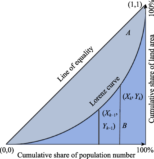
Figure 1 Illustration of Gini coefficient
where A+B is always 0.5, and thus Gini = 2A.
While the entire Lorenz curve is unknown, the values at certain intervals (here, by 2340 counties) are given. In this case, the Gini coefficient is approximated as
$Gini=\text{abs}\left( 1-\underset{k\text{=}1}{\overset{n}{\mathop \sum }}\,\left( {{X}_{k~}}-{{X}_{k-1}} \right)\left( {{Y}_{k}}+{{Y}_{k-1}} \right) \right)$
where n is the total number of counties, Xk and Yk are the cumulated percentages of population and land area for each county, respectively, and “abs” stands for absolute value as the Gini value is always positive.
The Gini coefficient value ranges 0-1 with 0 for minimum inequality and 1 for maximum inequality. A larger Gini coefficient indicates higher inequality.

2.3 Using REDCAP to derive the delineation line

As stated previously, we need to find a delineation line (similar to the Hu Line) that divides the study area into two parts that display the maximum disparity in population while possessing similar area sizes. This fits the classic task of regionalization, which groups (merges) small areas into regions that are homogenous within each region. We choose a GIS-automated regionalization method, termed “Regionalization with Dynamically Constrained Agglomerative Clustering and Partitioning (REDCAP)” by Guo (2008), to implement the task. Regions derived by the REDCAP method enjoy several advantages over other alternatives in spatial compactness, attribute homogeneity, and scale flexibility (Guo, 2008). Therefore, the application of REDCAP is becoming more and more popular (Benassi and Ferrara, 2010; Benassi et al., 2010; Jin et al., 2015).
The REDCAP method explicitly incorporates spatial contiguity constraints during the hierarchical clustering process, and optimizes an objective function (i.e., maximum homogeneity within regions) during the construction and partitioning of a cluster hierarchy to obtain a given number of regions. Specifically, REDCAP is composed of two steps. Step 1 starts merging two most similar and adjacent areas to form one region, and continues until all are merged into one region. A link marks each merger in the process. Dissimilarity between two neighboring areas i and j is measured by their attribute distance Dij such as
${{D}_{ij}}={{({{x}_{i}}-{{x}_{j}})}^{2}}$
where xi and xj are standardized attribute values for objects i and j. Step 2 reverses the order by removing a link that creates two regions with maximum homogeneity (or minimum heterogeneity) within them and continuing to remove the next link to generate more regions until a desirable number of regions are obtained. The overall heterogeneity is measured by the total sum of squared deviations (SSD) (Everitt, 2002), such as
$SSD=\sum\limits_{r=1}^{k}{\sum\limits_{i=1}^{{{n}_{r}}}{{{({{x}_{i}}-\bar{x})}^{2}}}}$
where k is the number of regions; nr is the number of small areas in region r; xi is a variable value; and $\bar{x}$ is the regional mean in region r. Readers are encouraged to consult the aforementioned references for more technical details.
More recent versions of the REDCAP accommodate additional constraints including threshold population in derived regions (Guo and Wang, 2011; Wang et al., 2012). This property makes it especially suitable for our study to define two regions with comparable area sizes.

3 Analysis of changes in population density and disparity at the county level

3.1 Examining population density changes

As shown in Table 1, the annual population growth rate has fluctuated since the first census in 1953. It increased from 13‰ in 1953 to 21‰ in 1982, and then began to decline to 7‰ in the year 2010. The rapid population growth from 1953 to 1982 benefited from the economic progress and social stability after the foundation of PRC. In addition, the family planning policy (or birth control campaign) was voluntary before the 1970s. Therefore, China experienced a rapid population growth period from the first census to the third one. Since the 1970s, the family planning policy transformed a voluntary birth control program into a mandatory program, and from late marriage and childbearing, birth spacing, and fertility limitation policy in the 1970s to one child policy in the 1980s (Attane, 2002). It resulted in a sharp descent in fertility rates, which explained the reason why the annual growth rate showed a continuous decreasing trend from 1982.
Table 1 Population changes between two census years in China
Census year Annual population growth rate (‰) Number of counties
With population decline With population growth
1953-1964 16 408 1,932
1964-1982 21 104 2,236
1982-1990 15 143 2,197
1990-2000 10 543 1,797
2000-2010 7 957 1,383
As for the population change in each county, 2340 counties are classified into five categories: very low density (0-100 people/km2), low density (101-200 people/km2), medium density (201-500 people/km2), high density (501-1000 people/km2), and very high density (>1000 people/km2). As shown in Figures 2a and 2b, in 1953, more than 1100 counties had population density less than or equal to 100 per/km2, covering more than 80% of the total land area. Both the number of counties and total area size for this very-low-density category declined significantly from 1953 to 1982, and then became relatively stable after that. This was consistent with the trend of population growth in general as the earlier part of the study period experienced rapid population growth and the later period was fairly stable. The numbers and areas for low-density and medium-density counties kept relatively stable for the entire study period. The number and land area of high-density counties had a noticeable and consistent growth trend from the year 1953 to 2000, and then began to decline from 2000 to 2010. The very-high-density counties, likely representing urban areas, accounted for small proportions in their number and land area. Both the number and land have been growing consistently over the entire period, and reached 216 counties and accounted for 1.8% of the total land area in 2010, reflecting the process of urbanization.
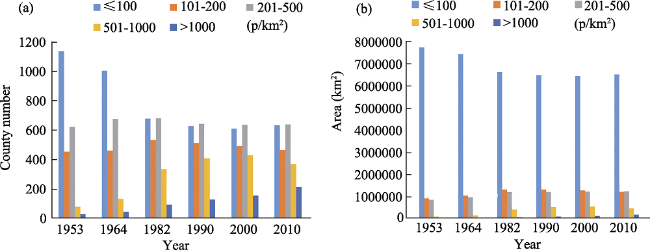
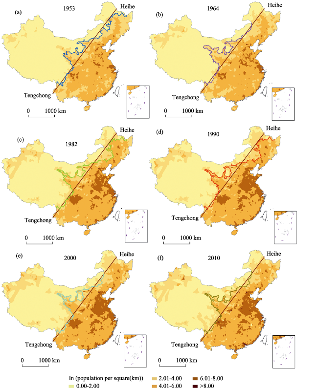
Figure 2 Distributions of population density at the county level 1953-2010 in China: (a) number of counties, (b) area size
Based on the per thousand (‰) annual population growth rates, the counties were classified into five grades: negative growth (≤0), minimal growth (0<R≤20), slow growth (20<R≤50), moderate growth (50<R≤100), and fast growth (R>100). Since the area size for each county remained constant over time, population growth rates were equivalent to population density growth rates. As shown in Figures 3a-3b and 4a-4b, for both periods of 1953-1964 and 1964-1982, most of the counties fell into the categories of minimal growth and slow growth. The moderate growth and fast growth counties also accounted for considerable proportions in both county number and area size as the country experienced rapid population growth overall, as stated previously. For 1982-1990 and 1990-2000, both the county number and size of minimal-growth counties were more than all the other combined, reflecting the national trend of gradually slowing down in population growth. For the most recent period 2000-2010, the minimal growth counties and negative growth counties accounted for the most proportion. The negative growth rate counties reached the largest number (957) among the five periods, as these counties lost population to urbanization. This was especially pronounced in large rural counties in eastern China (Liu et al., 2009), and left many villages in these counties depleted in population (Long et al., 2012) and some cases even extended to townships and cities observed (Long and Wu, 2016). Also noticeable were many counties in west China with moderate and fast growth rates in 1990-2000 and 2000-2010 (Figures 3d-3e). These low-density counties were rather small in population but large in area size, and the actual gains in population were modest.
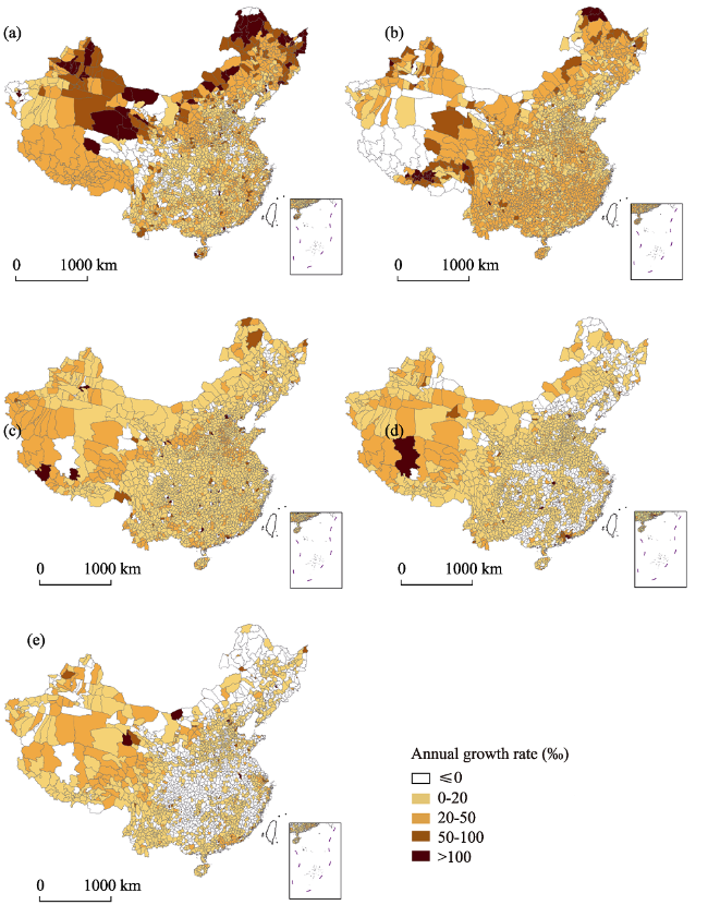
Figure 3 Population (density) growth rates at the county level in China
In short, over the study period, the number of fast-growth counties and their areas increased, so did the number and areas of negative-growth counties. In other words, the country became increasingly polarized in a contrast of population density as it underwent urbanization.
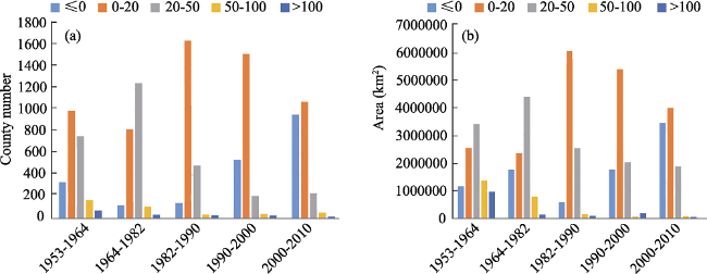
Figure 4 Distributions of population density growth rates at the county level 1953-2010 in China: (a) number of counties, (b) area size

3.2 Analysis of population density disparity by Gini coefficient

Gini coefficient is used here to further assess the outcome of aforementioned increasing gaps in population (density) growth rates. As shown in Table 2, the Gini values for the entire study period stayed above 0.65, indicating highly unequal population distributions in China.
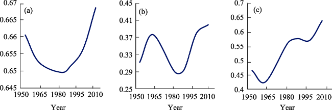
Table 2 Gini coefficients for disparity in population distribution in China
Census year Whole
country
Regions
Southeast Northwest
1953 0.661 0.316 0.467
1964 0.653 0.380 0.428
1982 0.650 0.294 0.563
1990 0.652 0.299 0.579
2000 0.657 0.382 0.573
2010 0.669 0.403 0.641
As illustrated in Figure 5a, the Gini coefficient for the entire country started out high in 1953, declined until reaching the valley bottom in 1982, and began an upward trend until 2010. The trend is characterized as a “U-shaped” pattern. The variation was confined to a narrow range 0.650-0.670, reflecting that the uneven distribution pattern in population was persistent.
Three possible forces help us understand the declining Gini values from 1953 to 1982.
One was the “Third Front Movement”, a massive industrial development by the central government in its interior from 1964 to 1976. During the period, national investment in industries and infrastructures focused in the mountainous inlands, considered safer than the east coastal areas for national defense. This movement supported significant government-sponsored migration in labor force. From late 1968 onward till 1976, another movement just as significant was the campaign termed “Up to the mountains, down to the villages.” Millions of urban youth were mobilized and sent to rural villages and frontiers for “reeducation.” Similarly, this brought much migration from more-urbanized and higher-density east coast to more primitive and lower-density inlands. Thirdly, when the draconian birth control policy was launched in the early 1970s, it was much harsher and more strictly enforced in the urban areas and residents were subject to the one-child policy. In rural areas, couples were allowed to have two children under certain conditions. Moreover, minority couples could have two or more children (Gu et al., 2007), and disproportionally high percentages of minorities were distributed in the southwest and west of China.
Figure 5 Gini coefficients for population density at the county level 1953-2010 in China: (a) the whole country; (b) southeast; (c) northwest
The reversed trend of increasing disparity after 1982 was attributable to the unpresented economic development in the era of economic reform and opening-up policy. During these periods, the east coastal regions experienced faster economic growth and urbanization than the rest of the country, and attracted massive migrant workers (Sun, 2013).

4 Analysis of population density disparity by regionalization

The previous section examines population density disparity and changes at the county level. While the analysis is at a fine geographic resolution, the variability is detailed, fragmented, and sometimes hard to detect patterns or trend. Geography is best learned at various scales. This section moves to analyze the same theme in a different scale. Instead of an analysis at the prefecture or provincial level (both administrative units are large than county), we seek to construct “organic” regions by a GIS-automated regionalization method, specifically REDCAP, and examine the disparity in population distribution by the derived regions. For the interest of validating the classic and influential Hu Line, this study is limited to delineate one demarcation line and generate two regions. Based on the six censuses, we are also interested in probing possible shifts of the demarcation line over time.

4.1 Population (density) disparity in regions divided by the Hu Line

As a baseline, Table 3 reports the population sizes and population densities in the two regions divided by the Hu Line in the six census years. Given similar area sizes (5.28 million km2 in the northwest and 4.17 million km2 in the southeast with a ratio of 55.9%: 44.1%), the contrast or disparity in population between the two regions divided by the Hu Line was very evident. The population ratio (southeast vs. northwest) declined from 95.78:4.22 in 1953 to 94.07:5.93 in 2010. The declining trend was consistent with the only exception that the ratio increased slightly from 1964 to 1982. In other words, disparity in population density between the southeast and northwest regions has been reduced. Given the large population size in the country, the 1.71% change in population proportion was very significant. For the counties along the Hu Line that are split, areal weighting interpolator was used to estimate their population in each side of the line proportionally to the corresponding area sizes.
Table 3 Population and population densities in regions divided by the Hu Line in China
Censusyear Whole country Southeast Northwest Population % ratio
(Southeast:
Northwest)
Population
(mil)
Population density(p/km2) Population
(mil)
Population density(p/km2) Population
(mil)
Population
density(p/km2)
1953 578.7 61.23 554,2 132.84 24.4 4.63 95.78 : 4.22
1964 689.7 72.98 658,4 157.80 31.3 5.93 95.46 : 4.54
1982 1,003.9 106.22 949,4 227.56 54.5 10.32 94.57 : 5.43
1990 1,130.5 119.61 1,067,8 255.93 62.7 11.88 94.45 : 5.55
2000 1,242.6 131.47 1,170,6 280.57 72.0 13.64 94.21 : 5.79
2010 1,327.4 140.44 1,248,6 299.27 78.7 14.92 94.07 : 5.93

4.2 Population (density) disparity in REDCAP-derived regions

The Hu Line divides China into two regions with comparable area sizes but significantly different population number. As stated previously, this study attempts to derive a demarcation line that divides China into two regions with maximum contrast in population, and examines the (in)consistency between this simulated line and Hu Line.
Empirical studies on regional population density patterns including China (e.g., Wang 2001) suggest that population densities usually decline exponentially with distances from cities. By extension, population density varies exponentially across space. Therefore, population density in logarithm was used to measure attributive homogeneity in implementing the REDCAP regionalization method (Wang et al., 2019). As shown in Figures 6a-6f, all six REDCAP-derived lines were largely consistent with the Hu Line and relative stable over time. One noticeable discrepancy is an area of relative higher density near the midpoint of the Hu Line (Guanzhong Basin) that falls in the northwest region by the Hu Line but the southeast region by the REDCAP line.
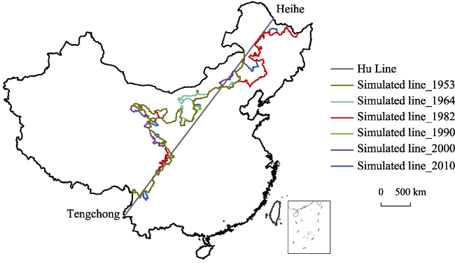
Figure 6 Two regions derived by REDCAP in China
Table 4 summarizes the population and land area proportions of two REDCAP-derived regions over time. All simulated lines divided the country into two regions with comparable area sizes but a striking difference in population. The regionalization for 1953, 1982, and 1990 yielded similar results as the southeast region smaller than the northwest (about 45% vs 55%). The regionalization for 1964, 2000, and 2010 yielded of near-identical area size. The expansion of area size in the southeast region was largely attributable to the significant increase in population density in the northwest corner in the Northeast China Plain (credited to the land cultivation campaign by massive state-owned farms and more recently turned agricorporations in the region) (Zuo, 2014), and pushed the simulated lines toward the west. The population ratios in the southeast for all the six censuses were between 97:3 and 98:2. In other words, the two regions by the REDCAP method had a much stronger contrast in population than those by the Hu Line. As the simulated lines can better capture the detailed variability in population density than the straight Hu Line, they revealed the disparity of population density pattern better than the Hu Line.
Table 4 Comparison of the two REDCAP-derived regions in China
Census years Southeast region Northwest region Difference
1953 Population (mil) 567.3 11.4 555.8
Population proportion (%) 98.03 1.97 96.06
Area (km2) 4308719.82 5142719.71 -833999.89
Area proportion (%) 45.59 54.41 -8.82
Population density (p/km2) 131.65 2.22 129.43
SSD 948.50
1964 Population (mil) 679.1 11.9 667.2
Population proportion (%) 98.3 1.7 96.6
Area (km2) 4921555.01 4529884.53 391670.48
Area proportion (%) 52.07 47.93 4.14
Population density (p/km2) 137.98 2.63 135.35
SSD 1104.71
1982 Population (mil) 973.0 31.0 942.0
Population proportion (%) 96.91 3.09 93.82
Area (km2) 4251784.34 5199655.19 -947870.85
Area proportion (%) 44.99 55.01 -10.02
Population density (p/km2) 228.84 5.96 222.88
SSD 1029.58
1990 Population (mil) 1096.3 34.2 1062.1
Population proportion (%) 96.97 3.03 93.94
Area (km2) 4276517.16 5174922.37 -898405.21
Area proportion (%) 45.25 54.75 -9.5
Population density (p/km2) 256.35 6.61 249.74
SSD 1034.87
2000 Population (mil) 1214.0 28.4 1185.6
Population proportion (%) 97.71 2.29 95.42
Area (km2) 4839160.69 4612278.85 226881.84
Area proportion (%) 51.20 48.80 2.4
Population density (p/km2) 250.87 6.16 244.71
SSD 1219.10
2010 Population (mil) 1292.9 34.5 1258.4
Population proportion (%) 97.40 2.60 94.8
Area (km2) 4799650.18 4651789.36 147860.82
Area proportion (%) 50.79 49.22 1.57
Population density (p/km2) 269.37 7.42 261.95
SSD 1351.82
As measured in equation (4), the total sum of squared deviations (SSD) captures the overall heterogeneity in the derived regions. Overall, the SSD value increased from 1953 to 2010 with a small peak in 1964. The increasing SSD value indicated enlarging disparity in population density across counties within the two regions (southeast and northwest regions) defined by the REDCAP method. This observation echoes the finding of a more polarized density pattern in China based on the increasing Gini coefficients reported previously in Table 2.
A closer examination on the movement of the simulated line over time, as shown in Fig- ures 6a-6f and Figure 7, reveals changes that are more detailed. Instead of toward one direction, it moved back and forth.
Figure 7 The overlapping of six simulated lines and the Hu Line in China
The following attempts to provide some insight into the underlying forces for the changes.
(1) For 1953-1964, the simulated line moved toward west, especially the northeast part. One likely cause was that immediately after the establishment of P. R. China, the central government followed the Soviet model in building up the heavy industry capacity. Much of the investment of industrialization in that era was concentrated in the northeast region, which brought a sizable migration there. The faster population growth rate in that area raised the population density there (also see Figure 3a), and helped push the demarcation line toward west.
(2) For 1964-1982, the simulated line moved to east, back to where the line stood in 1953. This period witnessed the fastest annual population growth in China (Table 1), but the uneven spatial distribution in growth rates (Figure 3b) in the northeast region increased the density gaps between the northwest corner and the rest of the region and shifted the delineation line eastward.
(3) For 1982-1990, the simulated line remained stable. After the economic reform and opening-up policy just took effect, the eastern coastal areas in China benefited first and its economic growth (mainly in urban areas) attracted some population (Lu et al., 2005; He et al., 2016). However, population migration was at its infancy stage, and the change was not enough to move the demarcation line.
(4) For 1990-2000, the line moved to west in the northeast part. One likely cause was the success of economic reform became more pronounced in the coastal provinces, and the magnitude of migrant workers increased a great deal towards large urban centers in the southeast for more job opportunities. This may help the expansion of higher-density areas in the southeast and push the line westward.
(5) For 2000-2010, the demarcation line remained the same as the trend in the previous period continued.
In addition, it is worthwhile to discuss the change of disparity within the southeast and northwest. As shown in Table 2 and Figures 5b-5c, the disparities within the two regions were much smaller than the whole country after much of the variability was already captured by the division between the two regions. Note that the southeast region always had a lower Gini value than the northwest. Within the southeast, the disparity exhibited a wavy variation (i.e., increasing in the beginning, then declining, finally increasing again). Within the northwest, the disparity showed an upward trend overall after 1963.

5 Conclusion

This research examines the spatial disparity in population distribution in China since the first official census in 1953. The traditional Gini coefficient is used to examine the variability and disparity of population density at the county level. The GIS-automated regionalization method, REDCAP, is used to divide China into two regions by a line similar to the classic Hu Line, and examines the disparity of population patterns on the two sides. Both approaches are applied to the analysis of census data over time to detect temporal trends.
Based on the Gini values derived from the county-level population data, the study finds that the disparity in population density declined from 0.661 in 1953 to 0.650 in 1982, but the trend was reserved with increasing Gini value from 0.650 in 1982 to 0.669 in 2010. The former was largely attributable to major political movements that emphasized equal economic development during the period, and the latter was a result of the economic reform and opening-up policy that led to the polarizing population settlement. The more recent trend since 1982 reflected the impact of urbanization that created fast-growing urban areas on the one side and declining rural areas on the other side. The dualism of increasingly crowded cities and more deserted countryside is likely to stay and further exacerbate in the foreseeable future.
Our examination of population distribution indicates that the disparity in population between the northwest and southeast regions separated by the Hu Line shrunk from 1953 to 2010. The northwest region accounted for slight over 4% of the country’s population in 1953 and increased to about 6% in 2010. By maximizing the difference in population density between two derived regions, we adopted the REDCAP method as a rigorous computation process to identify a demarcation (simulated) line in order to verify the classic Hu Line. This study has largely validated the Hu Line. The stability of the simulated line over time further supports the notion that this invisible barrier is tied to underlying factors such as physical environments suitable for human settlement, and is here to stay. The increasing SSD over time indicates an enlarged disparity within the southeast and northwest regions. In short, the trend in population distribution in China since 1953 experienced a minor reduction in disparity between the two mega-regions (southeast and northwest) while the heterogeneity within each increased.
[1]
Attane I , 2002. China’s family planning policy: An overview of its past and future. Studies in Family Planning, 33(1):103-113.

[2]
Benassi F, Bocci C, Petrucci A , 2010. Spatial data mining for clustering: From the literature review to an application using REDCAP. Working paper 2010/2011, Università degli Studi di Firenze.

[3]
Benassi F, Ferrara R , 2010. Regionalization with dynamically constrained agglomerative clustering and partitioning: An application on spatial segregation of foreign population in Italy at regional level. In: 45th Scientific Meeting of the Italian Statistical Society, Padova, 29.

[4]
Chen Z, Wang J, Ma G et al., 2013. China tackles the health effects of air pollution. The Lancet, 382(9909):1959-1960.

[5]
Everitt B S , 2002. The Cambridge Dictionary of Statistics. Cambridge University Press.

[6]
Goodchild M F, Lam N S-N , 1980. Areal interpolation: A variant of the traditional spatial problem. Geoprocessing, 1:297-331.

[7]
Gu B, Wang F, Guo Z et al., 2007. China’s local and national fertility policies at the end of the twentieth century. Population and Development Review, 33(1):129-148.

[8]
Guo D , 2008. Regionalization with dynamically constrained agglomerative clustering and partitioning (REDCAP). International Journal of Geographical Information Science Archive, 22(7):801-823.

[9]
Guo D, Wang H , 2011. Automatic region building for spatial analysis. Transactions in GIS, 15(Suppl.1):29-45.

[10]
Guo H, Wang X, Wu B et al., 2016. Cognizing population density demarcative Line (Hu Huanyong Line) based on space technology. S&T and Society, 31(12):1385-1394. (in Chinese)

[11]
He C, Chen T, Mao X et al., 2016. Economic transition, urbanization and population redistribution in China. Habitat International, 51:39-47.

[12]
Hu H , 1935. Distribution of China's population: Accompanying charts and density map. Acta Geographica Sinica, (2):33-74. (in Chinese)

[13]
Hu H , 1990. The distribution, regionalization and prospect of China’s population. Acta Geographica Sinica, 45(2):139-145. (in Chinese)

[14]
Huang R , 2005. Population redistribution in the context of urbanization in Beijing since 1980s. Population Research, (5):19-26.

[15]
Jin X, Zhang L, Gu J et al., 2015. Modelling the impacts of spatial heterogeneity in soil hydraulic properties on hydrological process in the upper reach of the Heihe River in the Qilian Mountains, Northwest China. Hydrological Processes, 29(15):3318-3327.

[16]
Liu C, Wang F, Xu Y , 2019. Habitation environment suitability and population density patterns in China: A regionalization approach. Growth and Change: A Journal of Urban and Regional Policy, 50:184-200.

[17]
Liu Y, Liu Y, Zhai R , 2009. Geographical research and optimizing practice of rural hollowing in China. Acta Geographica Sinica, 64(10):1193-1202. (in Chinese)

[18]
Long H, Li Y, Liu Y, Woods M, Zou J , 2012. Accelerated restructuring in rural China fueled by ‘increasing vs. decreasing balance’ land-use policy for dealing with hollowed villages. Land Use Policy, 29:11-22.

[19]
Long Y, Wu K , 2016. Shrinking cities in a rapidly urbanizing China. Environment and Planning A, 48(2):220-222.

[20]
Lorenz M O , 1905. Methods of measuring the concentration of wealth. Publications of the American Statistical Association, 9(70):209-219.

[21]
Lu Z, Huang Q H, Lu T et al., 2005. Process and problems of industrialization and urbanization in China. China Industrial Economy, 12:5-13.

[22]
Mao Q, Long Y, Wu K , 2016. Spatio-temporal changes of population density and urbanization pattern in China (2000-2010). China City Planning Review, 25(4):8-14.

[23]
Shan Z , 2009. China's mutant line: Hu Line. Chinese National Geography, (10):288-301. (in Chinese)

[24]
Sun Z , 2013. Explaining regional disparities of China’s economic growth: Geography, policy and infrastructure. Berkeley, CA: University of California.

[25]
The World Bank , 2007. Cost of pollution in China: economic estimates of physical damages. The World Bank, Washington, DC.

[26]
Wang F , 2001. Regional density functions and growth patterns in major plains of China, 1982-90. Papers in Regional Science, 80:231-240.

[27]
Wang F, Guo D, McLafferty S , 2012. Constructing geographic areas for cancer data analysis: A case study on late-stage breast cancer risk in Illinois. Applied Geography, 35(1/2):1-11.

[28]
Wang F, Liu C, Xu Y , 2019. Analyzing population density patterns in China with GIS-automated regionalization: The Hu Line revisited. Chinese Geographical Science, 29(4):541-552.

[29]
WHO, 2013. Country profile of environmental burden of disease: China.

[30]
Xue J , 1997. Urban-rural income disparity and its significance in China. Hitotsubashi Journal of Economics, 38(1):45-59.

[31]
Yu F, Ma G, Qi J et al., 2012. Report of China’s Environmental-economic Accounting in 2007-2008. Beijing: China Environmental Science Press. (in Chinese)

[32]
Yuan H , 1993. Study on the rationality of Chinese population distribution. Geographical Research, 12(3):64-69. (in Chinese)

[33]
Zuo M , 2014. China turning state-owned farms into agricorporations to take on world players. South China Morning Post (dated Aug 14, 2014). Available (last accessed 08-05-2019).

Outlines

/