Research Articles

Identifying the most important spatially distributed variables for explaining land use patterns in a rural lowland catchment in Germany

  • Chaogui LEI ,
  • Paul D. WAGNER ,
  • Nicola FOHRER
Expand
  • Institute for Natural Resource Conservation, Kiel University, Olshausenstr 75, 24118 Kiel, Germany

Chaogui Lei, M.Sc, E-mail: cglei@hydrology.uni-kiel.de

Received date: 2018-11-08

  Accepted date: 2019-02-21

  Online published: 2019-12-05

Copyright

Copyright reserved © 2019. Office of Journal of Geographical Sciences All articles published represent the opinions of the authors, and do not reflect the official policy of the Chinese Medical Association or the Editorial Board, unless this is clearly specified.

Abstract

Land use patterns arise from interactive processes between the physical environment and anthropogenic activities. While land use patterns and the associated explanatory variables have often been analyzed on the large scale, this study aims to determine the most important variables for explaining land use patterns in the 50 km² catchment of the Kielstau, Germany, which is dominated by agricultural land use. A set of spatially distributed variables including topography, soil properties, socioeconomic variables, and landscape indices are exploited to set up logistic regression models for the land use map of 2017 with detailed agricultural classes. Spatial validation indicates a reasonable performance as the relative operating characteristic (ROC) ranges between 0.73 and 0.97 for all land use classes except for corn (ROC = 0.68). The robustness of the models in time is confirmed by the temporal validation for which the ROC values are on the same level (maximum deviation 0.1). Non-agricultural land use is generally better explained than agricultural land use. The most important variables are the share of drained area, distance to protected areas, population density, and patch fractal dimension. These variables can either be linked to agriculture or the river course of the Kielstau.

Cite this article

Chaogui LEI , Paul D. WAGNER , Nicola FOHRER . Identifying the most important spatially distributed variables for explaining land use patterns in a rural lowland catchment in Germany[J]. Journal of Geographical Sciences, 2019 , 29(11) : 1788 -1806 . DOI: 10.1007/s11442-019-1690-2

1 Introduction

Land use and land cover affect the climate (Foley et al., 2005; Bonan et al., 2012), ecosystem structure (Ramachandran et al., 2018), hydrology and aquatic environment (DeFries and Eshleman, 2004), and thus have an impact on the development of the economy and population (Lambin and Meyfroidt, 2011). Throughout history, land use and land cover patterns have been diversified by urbanization, farmland expansion, and agricultural intensification (Lambin et al., 2001; Lawrence et al., 2008; Mustard et al., 2012). European agricultural land use has experienced considerable changes in the second half of the last century due to transformation in technology, socio-economy, and political management (Rounsevell et al., 2003). This has brought about considerable discrepancies in land use patterns. Heterogeneity of land use patterns affects several environmental aspects, such as air quality (Vleeshouwers and Verhagen, 2002), the distribution of the main components in the hydrological cycle (Neupane and Kumar, 2015), and biological diversity and ecosystem services (Alberti, 2005). Moreover, the economic development can be affected (Dissart and Vollet, 2011). Consequently, land use patterns are a multidisciplinary research topic that receives growing attention (Kok and Veldkamp, 2001; Zhang et al., 2013; Long and Qu, 2018; Ramachandran et al., 2018).
Since land use results from properties of the physical environment and from socio-economic development, relationships to biophysical and socio-economic spatially distributed variables are used to analyze land use change patterns (Mas et al., 2014; Aquilué et al., 2017). Relevant variables haven been used in a large number of land use change studies (Mitsuda and Ito, 2011). Properties of the environment, accessibility, socio-economic development, neighborhood and micro-policy variables are incorporated into statistical analyses like multiple linear regression or logistic regression, to study driving forces of urbanization (Deng et al., 2010; Shu et al., 2014). Among these variables, the relative importance of accessibility and socio-economic variables for urbanization has been shown (Liu et al., 2010). In contrast, spatial determinants that influence the location of agricultural land mostly relate to soil fertility, climatic patterns, or distance to markets (Mottet et al., 2006; Piquer-Rodriguez et al., 2018). These commonly used variables can be categorized as biophysical variables (e.g., topography, soil properties, climatic variables) and socio-economic variables (e.g., population density, distance to roads or villages, etc.), most of which have been used to predict spatial patterns of urban or agricultural land use change (Oñate-Valdivieso and Sendra, 2010; Baumann et al., 2011; Yang et al., 2014). Landscape metrics (like perimeter-area ratio) that quantify specific spatial characteristics of land patches represent land use heterogeneity in space (Inkoom et al., 2018). They manifest land use impact gradients (Fernandes et al., 2011), and are applied to land use modeling (Yang et al., 2014). Hence, landscape metrics have a potential to explain land use location, considering bidirectional connections between the land patch configuration and land use dynamics. In a particular region, the spatial pattern of one land use type is primarily shaped by a definite set of variables (van Meijl et al., 2006). The identification of important explanatory variables for spatial patterns of all land use classes facilitates a more efficient prediction of land use dynamics and allows for a better understanding of the land use system.
Studies about spatio-temporal characteristics and dynamics of agricultural land mostly focus on one lumped agricultural or cropland class (Li and Yeh, 2002; Piquer-Rodriguez et al., 2018). This is in part due to the accessibility of coarse agricultural classification data, e.g. from agencies (Feranec et al., 2010) or derived from remote sensing data (El-Kawy et al., 2011), as well as a predominant focus on the large scale (Etter et al., 2006). Several detailed classes are only rarely considered, e.g., in the study (Mehdi et al., 2018) which depicts separate spatio-temporal patterns of cereals, soybeans, corn, and oilseeds. The conservation of different spatial patterns of croplands enhances agricultural productivity (Semwal et al., 2004; Brandes et al., 2016). Cropland change is driven by a large number of influencing factors and differs from region to region (Mehdi et al., 2018). Müller et al. (2009) have examined the characteristics of cropland variation and cropland abandonment. However, in summary, the determinants of cropland patterns have not gained much attention, yet.
To address this research gap, we developed logistic regression models for 11 agricultural and three non-agricultural land use classes in the rural catchment of the Kielstau, Germany. We used biophysical and socioeconomic variables as well as landscape metrics to identify the most important determinants of land use patterns. In particular, this study focuses on three objectives: 1) to find the best variables to explain the distribution of each land use class, 2) to identify the most important explanatory variables for the land use pattern, and 3) to analyze competition between land use classes in the catchment.

2 Materials and methods

2.1 Study area

The Kielstau catchment (Figure 1) is a small rural catchment in northern Germany covering an area of 50 km2 (Fohrer et al., 2014; Wagner et al., 2018). It is a sub-basin of the Treene river. The mean annual precipitation and temperature are 893 mm and 8.3°C (DWD, 2009), respectively. The topography is comparatively even, with an elevation ranging from approx. 27 m to 78 m a.s.l. (Figure 1). Soils of Gleysol, Podzol, and Luvisol (Figure 1) dominating this catchment are mainly used as arable land, and grassland or pasture. Kielstau is the main river with a total length of approximately 17 km, flowing through Lake Winderatt about 5 km downstream from the river source. The Lake Winderatt is surrounded by protected areas that are mainly used for moderate grazing (Fohrer and Schmalz, 2012). The Kielstau re- ceives discharge from two main tributaries: the Moorau and the Hennebach. To secure agricultural productivity, subsurface tile drainages have been installed during land reallocation (Riedel and Polensky, 1987), which caused wide, drained areas that were estimated to cover 38% of the entire catchment (Fohrer et al., 2007).
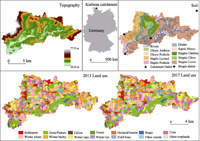
Figure 1 Location of the Kielstau catchment, spatial distribution of topography (LVA, 1992-2004), soil (BGR, 1999), main stream network (LANU, 2003), biogas plants, and land use in 2013 and 2017
Croplands constitute 63% of the study area and the majority is found in larger land patches as compared to the other land use classes. Among them, winter wheat, winter barley, winter rape, or corn take up a larger proportion, while winter rye, beans, oats, or row crops (sugar beet, potatoes, etc.) constitute a relatively smaller area. Crop rotations are commonly applied, resulting in constant changes within the croplands. Grassland or pasture (20%-21%) is mainly found in proximity to rivers and lakes or in protected areas. Urban, forest, water, and garden or orchard each occupy a smaller and persistent proportion.

2.2 Land use data

Land use maps of the years 2013 and 2017 (Figure 1) are used for spatio-temporal pattern analysis. The maps were acquired through field surveys in spring and early summer of 2013 and 2017. The main base data for this mapping process was extracted from the automated landed property map (ALK-Automatisierte Liegenschaftskarte, 2004) released by the state survey office of Schleswig-Holstein (LVERMA-SH). This map provides the outlines of all land patches. The land use class of every patch was mapped in the field. Furthermore, the consistency of the derived land use data was checked with the help of 0.2 m-resolution orthophotos (LVA, 2013, 2016) that were taken on 01/03/2013 and 26/08/2016.
Croplands comprise 62.8% in 2013 and 63.1% in 2017 of the catchment (Table 1). They are mainly classified into (1) cereals, including winter wheat, winter barley, winter rye, oats, and a smaller fraction of summer wheat and summer barley, (2) energy crops, like winter rape and corn silage, (3) row crops including potatoes and sugar beet, as well as (4) field bean, strawberries, and vegetables. With regard to semi-natural land use, grassland, meadow, mowing meadow, and pasture account for 20.8% in 2013 and 20.3% in 2017 (Table 1), respectively, and are primarily found along the rivers. The forest areas are nearly stable over time. Fallow areas are croplands that are not cultivated in the current year. It is mainly located in the southwestern region. Water areas cover approximately 1.8% including lakes, ponds, rivers and open creeks. Residential sites are located near main road intersections, with a slight increase from 10.5% in 2013 to 10.6% in 2017. Garden or orchard plots are scattered mostly near villages. To avoid very small land use classes and samples, the land use was divided into the following 14 main classes: settlement areas (residential, commercial, and industrial lands), fallow, grassland or pasture (field grass, meadow and pasture), corn, other croplands (strawberry, potato, sugar beet, etc.), forest, winter rye, winter rape, garden/orchard, winter wheat, other cereals (oats, summer wheat, summer barley), field beans, winter barley, and water.
Table 1 Areal percentages of land use classes in the Kielstau catchment in 2013 and 2017
Settlement
areas
Fallow Grassland
/Pasture
Corn Other
crops
Forest Winter rye Winter rape Orchard
/Garden
Winter wheat Other cereals Field
bean
Winter barley Water
2013 10.5 0.7 20.8 13.0 1.6 3.1 1.4 10.8 0.5 22.0 1.2 1.0 11.8 1.8
2017 10.6 0.6 20.3 10.7 2.1 3.1 3.5 11.8 0.5 21.4 2.0 2.4 9.2 1.8
Change 0.1 -0.1 -0.5 -2.3 0.5 0 2.1 1.0 0 -0.6 0.8 1.4 -2.6 0

2.3 Explanatory variables

Twenty-six spatially distributed variables have been used to explain the location of land use classes in space. Variables are depicted in Table 2, including topography variables, soil properties, distance and socioeconomic variables, and landscape metrics. All datasets are processed to a 10 m grid resolution. Spatial patterns of slope, silt content, drained soil share, distance to protected areas, population density, and fractal dimension are given as examples in Figure 2. Topography, soil properties, distance and socioeconomic variables are widely used to explain spatial patterns of land use and land use change (Verburg et al., 2004; Qasim et al., 2011). Landscape metrics have been previously used to quantify landscape structure and to assess land use and land cover change.
Figure 2 Examples of potentially important explanatory variables to land use distribution
A 5 m digital elevation model (DEM) derived from topographic map of Schleswig-Holstein (LVA, 1992-2004) has been used to generate elevation, slope, and aspect data at a 10-m resolution. The distance to roads or villages has been calculated from polygon roads and villages shapefiles that were extracted from land use maps in 2013 and 2017. The distance to rivers has been calculated from the main rivers shapefile of the Kielstau catchment (LANU, 2003). The distance to protected areas was derived based on the distribution of protected areas surrounding the Lake Winderatt and the Kielstau river (StiftungNaturschutz, 2016). By combining the land patch map with tile drained areas estimated (Fohrer et al., 2007), the percentage of drained area per patch was calculated. With regard to population density, (i) every 50 m2 settlement area is reclassified as one residential site based on a village map that was extracted from the land use map and from the digital basis landscape model (ATKIS-Basis-DLM) (LVA, 2016); (ii) residential sites are interpolated into a residence density raster using a Kernel algorithm (Silverman, 1981; Yan et al., 2011); (iii) the mean value of residents per site in each town is derived by dividing the number of inhabitants per town in June 2013 and December 2015 (Statistik Nord, 2013, 2015) by the amount of residential sites; (iv) the spatial population density is the product of the residence density raster with the mean value of residents per site. Soil properties are acquired from a combined application of soil type distribution derived from a Digital Soil Map (BGR, 1999) and soil attributes generated for a modeling study (Fohrer et al., 2014). As German biogas plants take in cereals, weeds, corn, and sunflowers as feedstocks (Golon, 2009), their distribution potentially affects crop distribution. Distance to biogas plants has therefore been considered and calculated according to the locations of two biogas plants within the catchment and another one near the catchment. Explicit outlines of land patches were extracted from land use maps in 2013 and 2017. Landscape metrics of all patches have been calculated with the Patch Analyst 3.1 extension for ArcGIS 10.3 and all other calculations have been carried out in ArcGIS 10.3.
Table 2 Spatially distributed explanatory variables used in this study
Variable Unit Source
Elevation m DEM for S.-H. (LVA, 1992-2004)
Aspect Degree Calculated from DEM
Slope Degree Calculated from DEM
Clay content % Digital soil map (BGR, 1999)
Silt content %
Sand content %
Rock content %
Organic carbon content %
Available water capacity mm/mm
Soil depth mm
Moist bulk density mg/m3
Saturated hydraulic conductivity mm/hr
Moist soil albedo -
USLE K factor -
Drained soil share %
Distance to rivers m Calculated from river network shapefile (LANU, 2003)
Distance to roads m Calculated from road distribution derived from 2013, 2017 land use maps
Distance to villages m Calculated from village distribution derived from 2013, 2017 land use maps
Distance to protected areas m Calculated from distribution of protected areas
(StiftungNaturschutz, 2016)
Distance to biogas plants m Calculated from biogas plants location
Population density Persons/km2 Calculated from community population and village distribution from 2013, 2017 land use maps
Patch size m2 Calculated from 2013 and 2017 land use maps
Patch perimeter m
Shape index -
Perimeter-area ratio m-1
Fractal dimension -

2.4 Logistic regression approach

Logistic regression models are used to analyze spatial patterns of all land use classes in the catchment with 26 explanatory variables (Table 2). Water areas are excluded from the analysis study as they occupy only a small proportion of the area. For each class C, a binary coding is employed, where 1 indicates the presence of class C; 0 indicates the presence of another class. The probability Pi for each pixel i (10m×10m) for the appearance of this land use class is calculated using a function of explanatory variables Xn,i as follows:
$log(\frac{P-{i}}{1- P-{i}})=\beta_{0}+\beta_{1}X_{1,i}+\beta_{2}X_{2,i}+\beta_{3}X_{3,i}+\beta_{4}X_{4,i}+\beta_{5}X_{5,i}$
where βn is the regression coefficient for the variable Xn,i. To seek the most important explanatory variables and avoid over-fitting, the number of explanatory variables n is limited to five. Previous studies also showed that five explanatory variables are sufficient to acquire reasonable results (Baumann et al., 2011; Wagner and Waske, 2016).
The relative operating characteristic (ROC) is used to assess model performance. The ROC statistic is the area under the curve of the rate of true positives versus the rate of false positives for a range of threshold values applied to the probabilities to achieve a binary classification. It ranges from 0.5 (random separation) to 1 (perfect discrimination) (Pearce and Ferrier, 2000). An ROC≥0.7 indicates that the independent variables have a strong capacity to model the dependent variable (Pontius and Schneider, 2001). In this study, the ROC value is used to select the model that is more suitable to explain land use patterns. To ensure that the selected variables are not collinear, Pearson’s correlation (r) is calculated for each variable pair. When r exceeds 0.7, the variable that better explains the land use appearance is retained and the other one removed (Baumann et al., 2011; Wagner and Waske, 2016). The logistic regression models of all possible combinations of five explanatory variables from non-collinear variable datasets are set up, by removing non-significant variables that are unable to optimize model performance according to a stepwise approach. Among these combinations, the 13 best logistic regression models with the highest ROC, one for each land use class, are selected and used for the analysis. To avoid spatial autocorrelation, for each specific land use class a stratified random sample is extracted by taking 20% of all pixels from its binary land use raster in 2017, and by excluding adjacent pixels in this sample (Wagner and Waske, 2016). The derived sample is randomly divided into two equal parts: one for calibration and one for validation of the models.
To assess the relative importance of the explanatory variables, all possible models derived from the calibration process by the ROC values are sorted and the first 50 best models for each class are selected. Then, how often each variable is included into these 50 models is counted. The percentage of the inclusion of a variable into best regression models is regarded as variable importance. All calculations, model executions, and analyses are performed in R and with the help of the R packages ROCR (Sing et al., 2005) and raster (Hijmans et al., 2016).

2.5 Validation and evaluation

The derived logistic regression models are quantitatively and visually evaluated in space and time (Pontius Jr et al., 2004). First, the validation half of the stratified random samples from the 2017 binary raster are used for spatial validation using the ROC statistic. Second, the model applicability is tested in time. To this end, some of the explanatory variables are updated: landscape metrics in 2013 are updated due to reshaped land parcels. Distance to villages is updated using slightly changed settlement areas in the 2013 land use map. Population density is recalculated by using village residence map and population data for the year 2013. The probabilities for each specific land use class in the entire catchment in 2013 are calculated, by applying the best logistic regression models to the 2013 explanatory variables. The derived probabilities are compared against the observed 2013 land use map with the help of the ROC statistic.
To further assess the plausibility of modeled results, R-G-B composites are used to visualize the competition for land in space between three different land use classes. An R-G-B composite is built by overlaying any three probability maps. In R-G-B composite maps, dark areas indicate low probabilities for these three classes, whereas light colors (near white) correspond to high probabilities for all of them, i.e. strong competition for land. Water areas are masked in white.

3 Results

3.1 Model performance

All explanatory variables that are included in the best logistic regression models are significant (p<0.05, Table 3). The best models are well above random discrimination as ROCs are greater than 0.5 (Table 3). The ROC for calibration (ROC_cal) ranges from 0.68 for corn to 0.97 for settlement areas. With regard to the spatial validation ROC values (ROC_val_2017) between 0.73 and 0.97 (Table 3) except for a slightly lower ROC of 0.68 for corn, are within the range of reliable precision 0.7-0.9 (Wu et al., 2009) or nearly 100% accurate with ROC value close to 1 (Pontius Jr and Schneider, 2001), highlighting reasonable performances of the derived models. Slightly lower ROC values from temporal validation (ROC_val_2013) indicate that the prediction of the 2013 land use pattern is a little worse (Table 3). Nevertheless, ROC_val_2013 values are greater than 0.71 with the exception of corn. The ROC for calibration differs from that for spatial validation and temporal validation by a maximum of 0.03 and 0.08, respectively. Hence, the derived regression models are reliable and robust both in space and in time. They can be used to accurately predict the spatial distribution of land use classes. Only corn is predicted with a slightly lower accuracy. Spatial patterns of croplands are often less accurately explained than non-croplands. For instance, ROCs for corn, winter wheat, and winter barley are equal to or smaller than 0.75, whereas ROCs for settlement areas, orchard/garden, fallow, and forest are equal to or larger than 0.84.
Table 3 Best logistic regression models for each land use class: odds ratios for the explanatory variables and performance of each model as indicated by the relative operating characteristic (ROC) statistic for calibration, spatial and temporal validation.

3.2 Variable impact

The majority of explanatory variables are included at least once in the best logistic regression models (Table 3). However, only few soil properties are used due to their higher collinearity, e.g. silt content has a positive correlation with soil organic carbon (r= 0.83) and clay content is negatively correlated with moist bulk density (r= -0.75). As only the variable that better explains land use appearance is included, soil organic carbon, available water capacity, and some other properties were not included in the best models (section 2.4).
The odds ratio, depicted as the value of exponent (βn) for the n-th variable, represent the impact of this variable on the predictor. The probability for land use presence will increase upon an increase in the n-th variable with odds ratio being greater than 1, whereas probability decreases with an increase in the variable when odds ratio is below 1. Table 3 shows that topography variables tend to affect natural or semi-natural land uses. Specifically, with an increase in slope by 1 degree the probability for fallow, forest, or orchard/garden appear to increase by 35.7%, 34.7%, and 50.3% (odds ratios=1.35698, 1.34681, 1.50291). When terrain ascends by 1 m, the probabilities for fallow and field beans decrease by 17.4% and 15.2% (odds ratios= 0.82567, and 0.84845, respectively).
Soil content variables (clay, silt, sand, or rock content) are mainly used to explain the occurrence of agricultural lands, e.g., with an increase of silt by 1%, winter wheat and winter barley become more probable by 8.9%, and 10.6%, respectively, and winter rye becomes less probable by 2.6%. Grassland or pasture is more probable on areas with a deeper first soil layer (0.2% increase per mm). The drained soil share affects seven land use classes. With an increase in the proportion of drained area by 1%, the probabilities for settlement, garden or orchard, and forest presence decrease by 3.4%, 2.4%, and 2.6%, respectively, while the probability for pasture increases 1.2%. Other crops (3.3%) and winter rye (1.3%) are less probable if the drained area share increases, whereas field beans are more probable (2.0%). The contrary effect on field beans is in agreement with the higher probability for field beans at low elevations, indicating that field beans are primarily found at lowland areas with a high drainage percentage in the catchment.
Distance variables and population density explain all land use classes. Particularly, distance to protected areas and population density are included in the best models for eight and five land use classes, respectively. As further away from protected areas, grassland or pasture becomes less probable (0.03% per meter, Table 3). In contrast, settlement areas and orchard or garden seem more probable (0.03%, 0.04% per meter, respectively) with increasing distance from protected area. There is no clear impact direction on croplands (Table 3). Population density has a clear effect on land use patterns; with an increase of one more person per square kilometer, settlement areas (0.4%) are more likely to be found, whereas fallow (0.9%), forest (0.8%), corn (0.3%), and other crops (0.3%) are less probable.
The influence of patch structure in particular of the fractal dimension is evidently different for croplands and non-croplands. An increase of fractal dimension indicating more complex patch shape (nearer 1 - simpler shape; 2 - irregular and complicated shape (Forman, 2014; Forman and Godron, 1981)) suggests that settlement area and forest (odds ratios > 1, Table 3) are more likely to be found on irregular patches, whereas croplands corn, winter rye, winter rape, winter wheat, other cereals, field beans, and winter barley all with odds ratios < 1 (Table 3) are more likely to be on simpler patches (e.g. large rectangles).

3.3 Variable importance

In addition to the best logistic regression model, the 50 best logistic regression models are derived for each land use class to evaluate the importance of explanatory variables. All models achieve a reliable performance with ROCs ranging from 0.72 to 0.97 except for corn (Table 4). Moreover, ROCs of the 50 best models only differ by a maximum of 0.03, indicating similar performance. The variables that are also included in the best model mostly have the greatest importance (percentages are marked in bold in Table 4). Some are even included in all of the 50 best models (100% inclusion). Overall, distance variables and population density are particularly important as they account for 31.7% of the variables that are used in these models, followed by soil properties (29.0%) and landscape metrics (28.7%), whereas topography (10.7%) is less important for rural land use patterns in this lowland region.
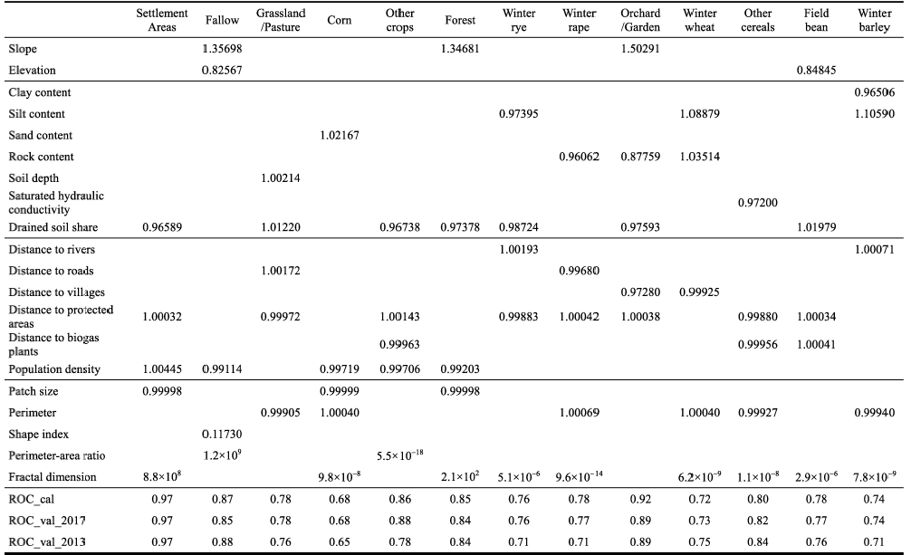
Table 4 Percentages of explanatory variables included into the 50 best logistic regression models for each land use class. The best model is marked in bold.
Distance to roads, distance to villages, distance to biogas plants, population density, and drained soil share are important for all land use classes, as they are at least included in two of the 50 best models (i.e. ≥4% inclusion, Table 4). Elevation, distance to protected areas, distance to villages, population density, drained soil share, perimeter-area ratio, and fractal dimension are of utmost importance as they are included at least one time in each 50 best models. Among them, patch fractal dimension (Pfd) is quite important for settlement areas (100% inclusion), mixed croplands (100% inclusion), field beans (96% inclusion), winter rye (88% inclusion), and forest (72% inclusion); distance to protected areas affects other croplands, winter rye, winter rape, and other cereals (inclusion ≥98%); drained soil share greatly explains the appearance of settlement areas, other croplands, forest, grassland, and field beans (inclusion ≥90%). Further important influences indicated by 100% inclusion are: elevation for fallow and field beans, distance to villages for orchard/garden, population density for forest, and patch perimeter-area ratio for other croplands.
In general, the variables distance to protected areas (mean inclusion 48%), population density (32%), drained soil share (51%), and patch shape complexity (fractal dimension, 66%) are largely important as they are more frequently included and used for 10 to 13 land use classes. Topography and soil properties contribute to fewer land use classes with a relatively low importance. The lower importance of topography is largely related to smaller terrain variations and similar potentials for crops throughout the catchment. The low impact of soil properties mainly results from the exclusion due to collinearity between soil variables, e.g. organic carbon content and moist bulk density are highly correlated with available water capacity (r= 0.84 and r= -0.85, respectively) and are, therefore, excluded as available water capacity is preferred during variables selection (Table 4). Nevertheless, soil properties indeed provide crucial information for the spatial distribution of cropland, e.g. silt content is an important explanatory variable for the spatial patterns of major cereals (winter rye 34%, winter wheat 98%, and winter barley 58%, respectively, Table 4) and part of the best model for these classes.

3.4 Analysis of probability maps of land use patterns

The probability maps for each land use class in 2013 are calculated using the best logistic regression model and the respective explanatory variables. For most of the land use classes, the spatial patterns of one or two defining explanatory variables show up clearly in their probability maps. For settlement areas, patterns of population density and drained area share are visible in the probability map: higher probability of settlement in areas of higher population density and lower percentages of drained area (Figures 2 and 3). Soil depth is part of the best model for grassland or pasture, and its outline is prevalent along the Kielstau river and to the east of Winderatt lake in the probability map for grassland. As a component of the best models for fallow and forest, the slope pattern is particularly visible in the southwestern part of the probability maps. For winter rye and winter barley, silt content is a determinative variable and results in clearly silt-analogous pattern in the probability maps. The probability map for orchard/garden exhibits a pattern similar to the variable distance to villages with higher likelihood nearer to villages. Other cereals are clustered near biogas plants, which is generally consistent with the surveyed distribution of other cereals in 2013 (Figure 1). The probability for field beans depends to a great degree on drained soil share. Field borders are explicitly visible in probability maps for all croplands, underlining the great importance of incorporating patch parameters into the cropland models.
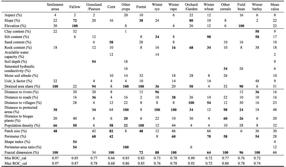
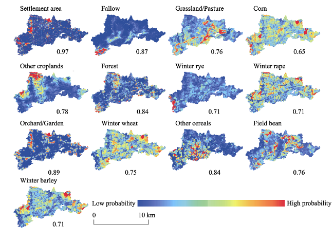
Figure 3 Probability maps for predicting each land use class pattern in 2013 using the best logistic regression models. The corresponding relative operating characteristic (ROC) statistic is provided.
R-G-B composite maps have been produced by overlaying probability maps to visualize competition between land use classes. From the composite map of settlement (Red, R), grassland/pasture (Green, G), and forest (Blue, B) as shown in Figure 4a, a majority of areas are found in these colors without mixing, i.e. settlement areas, grassland/pasture, and forest are well separated and do not compete for similar lands. In proximity to water areas, especially near the Kielstau River, green colors dominate indicating the high suitability for grassland or pasture. If the blue channel forest is replaced with winter wheat in Figure 4b, blue colors indicate the suitability for winter wheat. They are mostly found in areas with low probabilities for settlement, grassland/pasture and forest that are depicted in black in Figure 4a. The non-mixing colors red, green, and blue in Figure 4b can imply that no competition exists between dominant agricultural (e.g. winter wheat) and non-agricultural land use classes. In the R-G-B composites of the main croplands in Figures 4c and 4d, the probability maps of corn (R) or winter barley (R), winter rape (G), and winter wheat (B) are compared. An obvious feature is that mixed and light colors are prevailing in the two maps, suggesting that similar areas are simultaneously suitable for two or three crop types. Moreover, mixed colors present in the same patches in both composite maps represent the suitability of similar fields for these four main crops. Due to relatively high simulated probabilities for corn (depicted in red), more purple and magenta colors (mix of red and blue) are dominant in Figure 4c than in Figure 4d indicating higher probabilities for corn as compared to the competition of winter barley with winter wheat and winter rape. The cyan-blue colors dominating Figure 4d represent areas that are suitable for winter rape and winter wheat. The suitability of fields for different crop types is in agreement with crop rotations in the Kielstau catchment. The most common rotation is a mix of cereals and rapeseed, followed by a combination of corn and cereals, and of corn, cereals, and rapeseed (Kandziora et al., 2014).
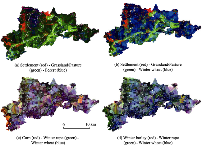
Figure 4 R-G-B composites indicating spatial competition among land use classes. Water areas are masked in white

4 Discussion

4.1 Most important explanatory variables

Our findings indicate which variables are important for the spatial distribution of land use classes in a small agricultural catchment in Germany. Most of these results are in agreement with our general understanding of the catchment. For instance, grassland or pasture have the highest probability near protected areas, the Kielstau river, and Lake Winderatt, which agrees with the principle that grassland or pasture instead of cropland is in direct vicinity to rivers to sustain water resource quality (Gerrish et al., 1995; Qureshi et al., 2013). Obviously, population density is a defining variable for settlement areas (Yue et al., 2013). Simpler patch shapes result in higher probability for croplands while more complex shapes are found in non-cropland areas. This is a reasonable result as crops are usually grown on larger and simpler fields as compared to other land use classes. The visual evaluation of the probability maps further confirms the plausibility of using the logistic regression models to simulate land use competition. The R-G-B composites of probability maps (Figure 4) indicate no strong competition between settlement areas, grassland/pasture, and croplands, which is reasonable in a rural environment that is not exposed to strong population pressure. However, the different crops (winter wheat, winter rape, corn, and winter barley) compete for the same locations, as indicated by the mixing and light colors in the both R-G-B composites of the probability maps Figures 4c and 4d. This is in agreement with the fact that these crops can be grown on the same fields. Crop variations are related to farmer decisions as well as to crop rotation practices of around three years that occur in the study area (Kandziora et al., 2014).
Our analysis shows that the most important variables to explain land use patterns in the Kielstau catchment are distance to protected areas, fractal dimension, drained soil share, and population density. These variables underline the agricultural character of the rural catchment, as fractal dimension, drainage density, and (low) population density are linked to agriculture. Moreover, the course of the Kielstau River affects the land use pattern as the variables distance to protected areas (Figure 2) and distance to rivers are linked to the Kielstau River, and the soil map includes properties of the flood plain (Figure 2). However, this may in part be explained by the fact that our analysis is carried out at the catchment scale. The logistic regression models are based on a dataset with a spatial resolution of 10 m. On a coarser spatial scale the spatial structure of the explanatory variables will be different and also the land use pattern will change, when smaller fields are merged. Consequently, other variables may be more important on the large scale. Nevertheless, we are confident that the 10 m resolution is appropriate for our comparatively small study area.

4.2 Model performance

The quantitative model performance as well as the visual evaluation of the probability maps (Figure 3) indicates that the derived logistic regression models can reasonably explain land use patterns in the Kielstau catchment. The patterns are overall consistent with the land use maps for 2013 and 2017 (Figure 1) and the ROC values for both spatial validation and temporal validation are mostly greater than 0.7 indicating a reasonable performance. The lowest ROC value for corn (0.65) may be attributed to the fact that corn cultivation is possibly more affected than other crops by non-spatial variables like market prices and policies as it may be used for biogas production. The assumption that corn fields can be found near biogas plants was not verified. This might also be explained by the small size of the study area and the small number of biogas plants.
The range of ROC values for the different land use classes can be explained by characteristics of rural land cover, e.g., settlement areas (0.97), orchard/garden (0.89), and forest (0.84) are well distinguished and thus have strong explanatory variables (e.g. population density, distance to villages, drained soil share, respectively), however, the explanatory variables are not similarly defining for one crop or the other and, therefore, yield lower accuracies with ROCs for most agricultural land between 0.7 and 0.8 in Table 3. In many other studies, agriculture is, therefore, only one lump class (Mottet et al., 2006; Yang et al., 2012), whereas this study differentiates eleven agricultural land use classes including eight cropland classes. A possible improvement could be achieved if the land tenure system was included as a spatial variable. This variable could be used to better represent farmers’ decisions as well as the influence of the market and policies.
A comparison of the model performances in 2013 and 2017 shows that the agricultural classes vary in time and that the performances differ, while they are more or less constant for non-agricultural classes. Usually, a slightly worse performance can be expected for temporal validation (Shu et al., 2014). This applies to winter rye, winter rape, and winter barley. But it has to be noted that some slight improvements for e.g. winter wheat and other cereals can be observed, indicating that the regression models fit the 2013 data moderately better. Since models are limited out at five explanatory variables it should not be neglected that if all significant variables are included better results can be achieved.

4.3 Value of landscape metrics for explaining land use patterns

Landscape metrics have been proven valuable in the context of our agricultural catchment. Hence, land patch structure and shape indicators are suitable to characterize and differentiate land use patterns, which is in agreement with the use of landscape metrics in the context of urban land use change or land cover classification studies (Seto and Fragkias, 2005; Fichera et al., 2012). Our results indicate that the landscape metrics provide important complementary information to the more commonly used biophysical and socioeconomic variables. Due to their explanatory power, they may also be useful in other study areas. The derived regression models are suitable to predict land use patterns and the derived probability maps can be used to visualize competition among land use classes in space, by incorporating the R-G-B composites as a simple model of land use competition. To simulate future land use patterns, the regression models can be incorporated into an intergrated application of CLUE-S (Liu et al., 2017) and Markov chain or cellular automata models (Arsanjani et al., 2013). These models also account for non-spatial variables like policy and market changes to alter the shares of different crops and derive a corresponding land use pattern.

5 Conclusion

A set of spatially distributed variables from topography, soil properties, distance variables and population density, and landscape metrics are derived to accurately explain land use patterns in the Kielstau catchment. From these categories, 20 variables contribute to the logistic regression models to explain the land use pattern. In particular, the explanatory variables distance to protected areas, drained soil share, patch fractal dimension, and population density are most important to characterize the land use distribution in space. These variables are either linked to agriculture or the river course of the Kielstau, which are identified as the two main influences for land use distribution in the catchment.
The derived models are suitable to explain and predict land use patterns. Both probability maps and ROC values between 0.71 and 0.97 for spatial and temporal validation underline this for all land use classes except that corn is harder to predict (ROC = 0.68, 0.65 for validation in space and in time, respectively). Non-agricultural classes are explained with higher precision, whereas the models for cropland classes yield lower performances. This result is mainly attributed to the fact that agricultural fields are usually suitable for more than one crop. Moreover, non-agricultural and agricultural classes are well distinguished in space, whereas dominant cropland classes compete mainly for the same land, so that modeling their distribution in space is particularly challenging. Competition between different classes can be explicitly and reasonably identified with probability maps and R-G-B composite maps of the main land use classes. The robustness of the models in space and in time indicates their potential for an inclusion in a combined modeling approach to produce land use patterns for future scenarios.

Acknowledgements

We gratefully acknowledge the financial support from the China Scholarship Council (CSC) through a scholarship for the first author. We thank three reviewers and the editor for their detailed and constructive comments that helped us to improve the manuscript.
[1]
Alberti M , 2005. The effects of urban patterns on ecosystem function. International Regional Science Review, 28(2):168-192.

[2]
Aquilué N, De Cáceres M, Fortin M J et al., 2017. A spatial allocation procedure to model land-use/land-cover changes: Accounting for occurrence and spread processes. Ecological Modelling, 344:73-86.

[3]
Arsanjani J J, Helbich M, Kainz W et al., 2013. Integration of logistic regression, Markov chain and cellular automata models to simulate urban expansion. International Journal of Applied Earth Observation and Geoinformation, 21:265-275.

[4]
Baumann M, Kuemmerle T, Elbakidze M et al., 2011. Patterns and drivers of post-socialist farmland abandonment in Western Ukraine. Land Use Policy, 28(3):552-562.

[5]
BGR, 1999. BUK 200, Bodenubersichtskarte 1:200 000. Bundesanstalt für Geowissenschaften und Rohstoffe: CC.1518 Flensburg, Hannover.

[6]
Bonan G B, DeFries R S, Coe M T et al., 2012. Land use and climate. In: Land Change Science. Dordrecht: Springer 301-314.

[7]
Brandes E, McNunn G S, Schulte L A et al., 2016. Subfield profitability analysis reveals an economic case for cropland diversification. Environmental Research Letters, 11(1):014009.

[8]
DeFries R, Eshleman K N , 2004. Land-use change and hydrologic processes: A major focus for the future. Hydrological Processes, 18(11):2183-2186.

[9]
Deng X, Huang J, Rozelle S et al., 2010. Economic growth and the expansion of urban land in China. Urban Studies, 47(4):813-843.

[10]
Dissart J C, Vollet D , 2011. Landscapes and territory-specific economic bases. Land Use Policy, 28(3):563-573.

[11]
DWD, 2009. Weather and Climate Data from the German Weather Service., Offenbach, Station Flensburg 1957-2006 and Station Meierwik, 1993-2008, 1993-2008 ed, Offenbach.

[12]
El-Kawy O A, Rød J, Ismail H et al., 2011. Land use and land cover change detection in the western Nile delta of Egypt using remote sensing data. Applied Geography, 31(2):483-494.

[13]
Etter A, McAlpine C, Wilson K et al., 2006. Regional patterns of agricultural land use and deforestation in Colombia. Agriculture, ecosystems & environment, 114(2-4):369-386.

[14]
Feranec J, Jaffrain G, Soukup T et al., 2010. Determining changes and flows in European landscapes 1990-2000 using CORINE land cover data. Applied Geography, 30(1):19-35.

[15]
Fernandes M R, Aguiar F C, Ferreira M T , 2011. Assessing riparian vegetation structure and the influence of land use using landscape metrics and geostatistical tools. Landscape and Urban Planning, 99(2):166-177.

[16]
Fichera C R, Modica G, Pollino M , 2012. Land Cover classification and change-detection analysis using multi-temporal remote sensed imagery and landscape metrics. European Journal of Remote Sensing, 45(1):1-18.

[17]
Fohrer N, Dietrich A, Kolychalow O et al., 2014. Assessment of the environmental fate of the herbicides flufenacet and metazachlor with the SWAT model. Journal of Environmental Quality, 43(1):75-85.

[18]
Fohrer N, Schmalz B , 2012. Das UNESCO Ökohydrologie-Referenzprojekt Kielstau-Einzugsgebiet-nachhaltiges Wasserressourcenmanagement und Ausbildung im ländlichen Raum (in German). Hydrologie und Wasserbewirtschaftung 56(4): 160-168.

[19]
Fohrer N, Schmalz B, Tavares F et al., 2007. Modelling the landscape water balance of mesoscale lowland catchments considering agricultural drainage systems. Hydrologie und Wasserbewirtschaftung/Hydrology and Water Resources Management-Germany, 51(4):164-169.

[20]
Foley J A, DeFries R, Asner G P et al., 2005. Global consequences of land use. Science, 309(5734):570-574.

[21]
Forman R T , 2014. Land Mosaics: The Ecology of Landscapes and Regions(1995). Island Press..

[22]
Forman R T, Godron M , 1981. Patches and structural components for a landscape ecology. BioScience, 31(10):733-740.

[23]
Gerrish J, Peterson P, Morrow R , 1995. Distance cattle travel to water affects pasture utilization rate. American Forage and Grassland Council.

[24]
Golon J , 2009. Enviromental Effects of varied Energe Crop Cultivation Scenarios on a Lowland Catchment in Northern Germany A SWAT Approach,Thesis (Master), Ecology Centre. Kiel University.

[25]
Hijmans R, van Etten J, Cheng J et al., 2016. Package ‘raster’: Geographic data analysis and modeling. R version 2. 5-8.

[26]
Inkoom J N, Frank S, Greve K et al., 2018. Suitability of different landscape metrics for the assessments of patchy landscapes in west Africa. Ecological Indicators, 85:117-127.

[27]
Kandziora M, Dörnhöfer K, Oppelt N et al., 2014. Detecting land use and land cover changes in northern German agricultural landscapes to assess ecosystem service dynamics. Landscape Online, 35.

[28]
Kok K, Veldkamp A , 2001. Evaluating impact of spatial scales on land use pattern analysis in Central America. Agriculture, Ecosystems & Environment, 85(1-3):205-221.

[29]
Lambin E F, Meyfroidt P , 2011. Global land use change, economic globalization, and the looming land scarcity. Proceedings of the National Academy of Sciences, 108(9):3465-3472.

[30]
Lambin E F, Turner B L, Geist H J et al., 2001. The causes of land-use and land-cover change: Moving beyond the myths. Global environmental change, 11(4):261-269.

[31]
LANU, 2003. LANDESAMT FÜR NATUR UND UMWELT SCHLESWIG-HOLSTEIN: Ausschnitt aus dem Basisgewässernetz des Landes Schleswig-Holstein für das Einzugsgebiet der Treene bis Treia. (Arc-View- Shape), Flintbek.

[32]
Lawrence D, D'Odorico P, Diekmann L et al., 2007. Ecological feedbacks following deforestation create the potential for a catastrophic ecosystem shift in tropical dry forest. Proceedings of the National Academy of Sciences, 104(52):20696-20701.

[33]
Li X, Yeh A G O , 2002. Neural-network-based cellular automata for simulating multiple land use changes using GIS. International Journal of Geographical Information Science 16(4):323-343.

[34]
Liu G, Jin Q, Li J et al., 2017. Policy factors impact analysis based on remote sensing data and the CLUE-S model in the Lijiang River Basin, China. Catena, 158:286-297.

[35]
Liu J, Zhang Z, Xu X et al., 2010. Spatial patterns and driving forces of land use change in China during the early 21st century. Journal of Geographical Sciences, 20(4):483-494.

[36]
Long H, Qu Y , 2018. Land use transitions and land management: A mutual feedback perspective. Land Use Policy, 74:111-120.

[37]
LVA, 1992-2004. DEM 25 m Grid Size, DEM 5 m Grid Size Derived from Topographic Maps 1:5 000 and Map of Schleswig-Holstein. Land survey office Schleswig-Holstein: Kiel.

[38]
LVA, 2013, 2016. ATKIS®-Digitale Orthophotos (DOP) with a ground resolution of 20 cm. Land Survey Office Schleswig-Holstein.

[39]
LVA, 2016. ATKIS® Digitales Basis-Landschaftsmodell (Basis-DLM). Land Survey Office Schleswig-Holstein: Kiel.

[40]
LVERMA-SH, Vermessungs-und Katasterverwaltung Schleswig-Holstein, 2004. Automatisierte Liegenschaftskarte (ALK).

[41]
Mas J F, Kolb M, Paegelow M et al., 2014. Inductive pattern-based land use/cover change models: A comparison of four software packages. Environmental Modelling & Software, 51:94-111.

[42]
Mehdi B, Lehner B, Ludwig R , 2018. Modelling crop land use change derived from influencing factors selected and ranked by farmers in North temperate agricultural regions. Science of The Total Environment, 631:407-420.

[43]
Mitsuda Y, Ito S , 2011. A review of spatial-explicit factors determining spatial distribution of land use/land-use change. Landscape and Ecological Engineering, 7(1):117-125.

[44]
Mottet A, Ladet S, Coqué N et al., 2006. Agricultural land-use change and its drivers in mountain landscapes: A case study in the Pyrenees. Agriculture, Ecosystems & Environment, 114:296-310.

[45]
Mustard J F, Defries R S, Fisher T et al., 2012. Land-use and land-cover change pathways and impacts. In: Land Change Science. Dordrecht: Springer, 411-429.

[46]
Müller D, Kuemmerle T, Rusu M et al., 2009. Lost in transition: Determinants of post-socialist cropland abandonment in Romania. Journal of Land Use Science, 4(1/2):109-129.

[47]
Neupane R P, Kumar S , 2015. Estimating the effects of potential climate and land use changes on hydrologic processes of a large agriculture dominated watershed. Journal of Hydrology, 529:418-429.

[48]
Oñate-Valdivieso F, Sendra J B , 2010. Application of GIS and remote sensing techniques in generation of land use scenarios for hydrological modeling. Journal of Hydrology, 395(3/4):256-263.

[49]
Pearce J, Ferrier S , 2000. Evaluating the predictive performance of habitat models developed using logistic regression. Ecological Modelling, 133(3):225-245.

[50]
Piquer-Rodriguez M, Butsic V, Gärtner P et al., 2018. Drivers of agricultural land-use change in the Argentine Pampas and Chaco regions. Applied Geography, 91:111-122.

[51]
Pontius Jr R G, Huffaker D, Denman K , 2004. Useful techniques of validation for spatially explicit land-change models. Ecological Modelling, 179(4):445-461.

[52]
Pontius Jr R G, Schneider L C , 2001. Land-cover change model validation by an ROC method for the Ipswich watershed, Massachusetts, USA. Agriculture, Ecosystems & Environment, 85(1-3):239-248.

[53]
Qasim M, Hubacek K, Termansen M et al., 2011. Spatial and temporal dynamics of land use pattern in District Swat, Hindu Kush Himalayan region of Pakistan. Applied Geography, 31(2):820-828.

[54]
Qureshi M E, Hanjra M A, Ward J , 2013. Impact of water scarcity in Australia on global food security in an era of climate change. Food Policy, 38:136-145.

[55]
Ramachandran R M, Roy P S, Chakravarthi V et al., 2018. Long-term land use and land cover changes (1920-2015) in Eastern Ghats, India: Pattern of dynamics and challenges in plant species conservation. Ecological Indicators, 85:21-36.

[56]
Riedel W, Polensky R , 1987. Umweltatlas für den Landesteil Schleswig. Forschungsprojekt des Institutes für Regionale Forschung und Information im Deutschen Grenzverein e.V. in Zusammenarbeit mit der Zentralstelle für Landeskunde des Schleswig-Holsteinischen Heimatbundes.

[57]
Rounsevell M D A, Annetts J E, Audsley E et al., 2003. Modelling the spatial distribution of agricultural land use at the regional scale. Agriculture, Ecosystems & Environment, 95(2/3):465-479.

[58]
Semwal R L, Nautiyal S, Sen K K et al., 2004. Patterns and ecological implications of agricultural land-use changes: A case study from central Himalaya, India. Agriculture, Ecosystems & Environment, 102(1):81-92.

[59]
Seto K C, Fragkias M , 2005. Quantifying spatiotemporal patterns of urban land-use change in four cities of China with time series landscape metrics. Landscape Ecology, 20(7):871-888.

[60]
Shu B, Zhang H, Li Y et al., 2014. Spatiotemporal variation analysis of driving forces of urban land spatial expansion using logistic regression: A case study of port towns in Taicang City, China. Habitat International, 43:181-190.

[61]
Silverman B W , 1981. Using kernel density estimates to investigate multimodality. Journal of the Royal Statistical Society. Series B (Methodological), 97-99.

[62]
Sing T, Sander O, Beerenwinkel N et al., 2005. ROCR: Visualizing classifier performance in R. Bioinformatics, 21(20):3940-3941.

[63]
Statistikamt Nord S.A.f.H.u.S-H , 2013, 2015. Bevölkerung der Gemeinden in Schleswig-Holstein 2. Quartal 2013; Bevölkerungsentwicklung in den Gemeinden Schleswig-Holsteins 2015.

[64]
StiftungNaturschutz, 2016. Flächenmanagement Kreis SL-Stiftung Naturschutz Schleswig-Holstein.

[65]
Ulrich U, Hörmann G, Unger M et al., 2018. Lentic small water bodies: Variability of pesticide transport and transformation patterns. Science of the Total Environment, 618:26-38.

[66]
van Meijl H, Van Rheenen T, Tabeau A et al., 2006. The impact of different policy environments on agricultural land use in Europe. Agriculture, Ecosystems & Environment, 114(1):21-38.

[67]
Verburg P H, van Eck J R R, de Nijs T C M et al., 2004. Determinants of land-use change patterns in the Netherlands. Environment and Planning B: Planning and Design, 31(1):125-150.

[68]
Vleeshouwers L M, Verhagen A , 2002. Carbon emission and sequestration by agricultural land use: A model study for Europe. Global Change Biology, 8(6):519-530.

[69]
Wagner P D, Hoermann G, Schmalz B et al., 2018. Characterisation of the water and nutrient balance in the rural lowland catchment of the Kielstau (in German). Hydrologie und Wasserbewirtschaftung, 62(3): 145-158.

[70]
Wagner P D, Waske B , 2016. Importance of spatially distributed hydrologic variables for land use change modeling. Environmental Modelling & Software, 83:245-254.

[71]
Wu X, Hu Y, He H S et al., 2009. Performance evaluation of the SLEUTH model in the Shenyang metropolitan area of northeastern China. Environmental Modeling & Assessment, 14(2):221-230.

[72]
Yan Q, Bian Z, Zhang P et al., 2011. Spatialization of population density based on residential spots density. Geography and Geoinformatics, 27:95-98. (in Chinese)

[73]
Yang X, Zheng X Q, Chen R , 2014. A land use change model: Integrating landscape pattern indexes and Markov-CA. Ecological Modelling, 283:1-7.

[74]
Yang X, Zheng X Q, Lv L N , 2012. A spatiotemporal model of land use change based on ant colony optimization, Markov chain and cellular automata. Ecological Modelling, 233:11-19.

[75]
Yue W, Liu Y, Fan P , 2013. Measuring urban sprawl and its drivers in large Chinese cities: The case of Hangzhou. Land Use Policy, 31:358-370.

[76]
Zhang P, Liu Y, Pan Y et al., 2013. Land use pattern optimization based on CLUE-S and SWAT models for agricultural non-point source pollution control. Mathematical and Computer Modelling, 58(3/4):588-595.

Outlines

/