Habitat loss and fragmentation was considered as the main reason of plant biodiversity loss (Wilson et al., 2016), and the biodiversity pattern in medium and larger scale can be estimated by integrated analysis of habitat maps with threat factors (Fahrig, 2003; Tallis et al., 2013; Wilson et al., 2016), InVEST model introduced the habitat quality as a proxy for biodiversity assessment (Polasky et al., 2011; Tallis et al., 2013). Habitat quality was a function determined by four factors (e.g. each threat’s relative impact, the relative sensitivity of each habitat type to each threat, the distance between habitats and sources of threats, and the degree to which the land was legally protected (Tallis et al., 2013; Chen et al., 2016). Generally, habitat quality degradation was caused by the intensity of nearby land-use expansion related to human activities and land use/cover change (Xu et al., 2013; Liang and Liu, 2017). At the pixel scale, a pixel cell threat level was translated into a habitat quality using the total threat level and a half saturation function. The specific calculation formula was listed as follows:

$$Qxj=Hj\times \left[ 1-\left( \frac{Dx{{j}^{z}}}{Dx{{j}^{z}}+{{k}^{z}}} \right) \right]\ \ \ \ \ (1)$$

$$Dxj=\sum\nolimits_{r=1}^{R}{\sum\nolimits_{y=1}^{{{Y}_{r}}}{\left( {{{W}_{r}}}/{\sum\limits_{r=1}^{R}{{{W}_{r}}}}\; \right)}}{{r}_{y}}{{i}_{rxy}}{{\beta }_{x}}{{S}_{jr}}\ \ \ \ (2)$$

where Q_xj is ecological habitat quality value of land use type j, H_j is a habitat quality score that ranges from 0 to 1, where non-habitat land-use types are given a score of 0 and perfect habitat classes are scored 1, D_xj is the total threat level in grid cell x with land-use type j, and k is the half saturation constant (Tallis et al., 2013; Liang and Liu, 2017; Sun et al., 2015), Z is a constant. R is the number of ecological threat factor, W_r is the threat weight that relates destructiveness of a degradation source to all habitats, Y_r is the set of grid cells on r raster map, y is all grid cells, r_y is raster map r, i_rxy is the distance function of habitat quality and ecological threat factor, β_x is the level of accessibility in grid cell x, where 1 indicated complete accessibility; S_jr is the sensitivity of land use type j (habitat type) to the ecological threat factor r. Here, the accessibility of each land use type was equal according to the national laws without considering of land reserve difference in the BLJW. At the same time, the values of relative sensitivity S_jr of each habitat type to each ecological threat ranged from 0 to 1, where 1 represented high sensitivity to a threat and 0 represented no sensitivity to a threat (Xu et al., 2013; Liang and Liu, 2017). According to the natural system conditions and the current situation of BLJW, urban, rural residential areas, population density, cropland, roads, ecological risk source is selected as the main ecological threats (Table 1). In our study, primary roads refer to the national highways and provincial roads, the secondary roads refer to county and township roads, respectively; while the ecological risk source including landslide, debris flow, soil erosion, earthquake and drought. Then, the maximum effected distance of each ecological threat of urban, rural residential area, cropland, population density, primary roads, the secondary roads and ecological risk source are 6.0, 2.5, 1.5, 3.5, 2.5, 0.5, and 3.0 km, respectively. And the weight of each ecological threat of urban, rural residential area, cropland, population density, primary roads, the secondary roads and ecological risk source are 0.8, 0.4, 0.6, 0.3, 0.6, 0.5 and 1 according to the previous relative research results (Tallis et al., 2013; Xu et al., 2013; Sun et al., 2015; Wilson et al., 2016; Zhang et al., 2017; Liang and Liu, 2017) and the users` guide of InVEST model (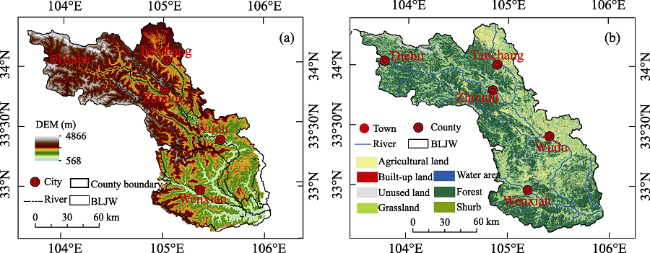Tallis et al., 2013), respectively. In this paper, Landsat TM/ETM+ images (nominal resolution is 30 m×30 m, acquired on 9/1990 and 10/2010) are processed using the ENVI 4.8 software, which involves geometric correction, image enhancement and supervised classification (Du et al., 2016). Based on this, land cover dataset is obtained by supervised classification and visual image interpretation based on experimental knowledge and field observation, and land-use types are classified as agricultural land (AL) (including farmland, vegetable plots, orchards, and nurseries), forest land (FL) (including forest, spinney, open woodland, other forest), shrubs, grassland (GL) (including high, medium, low coverage grassland), built-up land (BL) (including residential, commercial, and industrial land together with public transportation corridors, and construction sites), water areas (WA) (including rivers, aqueducts, lakes, ponds, and reservoirs), and unused land (UL) (including salinized land, derelict land, bare land and low-coverage grassland with vegetation cover <5%). In addition, a total of 200 points are randomly selected to verify the precision of classification through field surveys, while the topographic map and images from Google earth with high spatial resolution are used as the accessorial materials, and the overall accuracies of the years 1990 and 2010 are both larger than 84%. Meanwhile, local residents are also interviewed about the land use history, and land transformation information provided by the local government is analyzed to understand and explain the factors responsible for triggering landscape changes. Finally, the other detailed input data for InVEST habitat quality model in the study are prepared. At the same time, due to different vegetation types had provided different habitat, the differences of vegetation types should be considered to the weight of habitat quality, respectively (Table 1).

Generally, the decline in NPP could indirectly reflect vegetation degradation and biodiversity reduction (Liu et al., 2015; Lausch et al., 2016) in the farming-grazing transitional region from the northern subtropical zone to the warm-temperate zone. BLJW was just located in this region of China, so NPP of BLJW could reflect the vegetation ecosystem production capacity, quality, elastic and biodiversity (Liu et al., 2015). Secondly, landscape structure index (LSI) referred to the landscape structure situation and played an important role in evaluating regional ecosystem sustainable development ability and landscape diversity. Generally, LSI could be calculated by the formulas listed below (Zhao, 2012; Xie et al., 2017):

$$LS{{I}_{x}}=1-(aCi+bNi+cFi)\ \ \ \ \ (3)$$

$$Ci=\frac{ni}{Ai}\ \ \ \ \ (4)$$

$$Ni=0.5\sqrt{{ni}/{A}\;}\times \frac{A}{Ai}\ \ \ \ \ (5)$$

$$Fi=2\ln \left( \frac{Pi}{4} \right)\ln Ai\ \ \ \ \ (6)$$

where LSI_x is landscape structure index, C_i is landscape fragmentation index, N_i is landscape separation index, F_i is landscape fractal dimension index, a, b and c represent the weights of the three indexes, P_i is the perimeter of patch i, n_i and A_i are the number of patches in the landscape and total landscape area of patch type i.

Here Q_xj, NPP and LSI, which refer to regional biological habitat quality, vegetation production capacity and landscape diversity, respectively, are used to obtain the comprehensive index of plant biodiversity spatial patterns, and can be expressed as the biodiversity index (BI_x):

$$B{{I}_{x}}={{Q}_{xj}}\times {{\beta }_{1}}+NP{{P}_{x}}\times {{\beta }_{2}}+LS{{I}_{x}}\times {{\beta }_{3}}\ \ \ \ \ (7)$$

where BI_x is plant biodiversity comprehensive index; β₁, β₂ and β₃ are the weights of Q_xj, NPP_x and LSI_x, respectively, which is calculated by Analytic Hierarchy Process (AHP). Based on the comprehensive consideration of the influence degree of each index of biodiversity pattern of BLJW and the previous researches to construct the comparison matrix, to calculate and obtain the maximum eigenvalue of comparison matrix (value of 3.09) and its feature vector, the value of CR was 0.042 < 0.1 through the consistency check.

As shown in Figure 2, the spatial distribution of habitat quality was changed obviously in BLJW. The low habitat quality area distributed widely and concentrated in the valleys of the BLJW between Zhouqu-Wudu-Wenxian counties, most of Tanchang County, and the northern part of Wenxian County, where human activities were relatively frequent and intensive. The higher habitat quality areas were mainly distributed in the mountain forest and nature reserves, such as Baishuijiang National Nature Reserve. On the administrative unit, habitat quality can be ranked as: Diebu County > Wenxian County > Zhouqu County > Tanchang County > Wudu District. During the period of 1990-2010, the habitat quality tended to increase, and the area proportion of high habitat quality increased from 20.2% to 25.4% while the area proportion of low habitat quality decreased gradually (Figure 2).

The average annual value and the highest value of NPP in BLJW were 500.59 gCm^-2a^-1 and 1147.68 gCm^-2a^-1 from 2001 to 2010, respectively. The low NPP areas located in the BLJ valley, hilly area, and alpine mountainous area which elevation was above 3500 m, while the high NPP areas were mainly distributed in Diebu County, Wenxian County, Duoer-Axia Nature Reserve (DNR-ANR), Chagangliang Nature Reserve (CNR), Dieshan Mountain Forest District (DMF) and Gaolou Mountain. On the other hand, the distributionpattern of LSI was similar with that of habitat quality and NPP. The areas with low LSI mostly located along Bailongjiang and its tributaries, the northwestern part of Tanchang County and the northern mountainous areas of Diebu County (such as Majie township, Anhua township, Hanwang township, Liangshui township, etc.), while the high LSI area distributed in the nature reserve and forestry areas (Figure 3). The average annual value of LSI in the BLJW had increased from 0.692 in 1990 to 0.696 in 2010.

Table 2 and Figure 4 display the BI change in BLJW from 1990 to 2010. During 1990-2010, the mean BI of BLJW increased from 0.28 in 1990 to 0.29 in 2010. The high biodiversity area increased obviously and its area proportion changed from 14.13% to 17.15%. The area proportion of medium-low and lower BI decreased which indicated that the biodiversity restoration in BLJW was still a huge challenge and needs to be paid more attention in the future. Spatially, the areas with high BI were mainly concentrated in the nature reserve areas, the middle and subalpine forest areas (Figure 4) which usually had a high vegetation coverage, better habitat quality, richer species, and were the key areas of rare animals and plants, such as Ailuropoda melanoleuca, Rhinopithecus roxellana, Antidorcas marsupialis, Elaphodus cephalophus, Acer paxii Franch, Davidia involucrata Baill, Metasequoia glyptostroboides, Cathaya, Toona ciliata Roem. The moderate BI areas mainly distributed in forest, shrub and grassland, and accounted for 45.18% of the watershed area, while the medium-low biodiversity area accounted for 28.88%. The proportion of low biodiversity was up to 8.79%, and mainly concentrated in farmland, mining area, urban and rural areas, disaster prone area and bare rock zones (Table 2 and Figure 4). Generally, as to the areas with lower BI value, the ecosystems characterized with less species, higher landscape fragmentation, fragile ecological environment, and/or frequent and intensive human disturbance.

Figure 5 showed that the high and moderate biodiversity areas mainly concentrated in the altitude range of 1400-3500 m, while the low biodiversity areas concentrated under the altitude of 1700 m or the higher altitude zone. At the same time, field surveys also found that the area of increasing biodiversity index mainly belonged to ecological engineering restoration area, natural protection and forestry areas, particularly the areas of Grain for Green Project, Natural Forest Protection Project, Shelter Forest Project in the middle and upper reaches of the Yangtze River, while the area where biodiversity decreasing located in the region with intensive and frequent human activities. Moreover, the areas with plant biodiversity improvement were larger than that of plant biodiversity reduction (or degradation), suggesting that the ecological environment and biodiversity were getting better in the BLJW recently.

Plant biodiversity has obvious spatial pattern variations in BLJW, and the lower biodiversity areas mainly distributed in farmland, urban and rural areas, bare land and the lower coverage grassland, while the high and high-moderate areas mainly distributed in the National Nature Reserve and forestry area. Specifically, the higher plant biodiversity area mainly distributed in six sub-regions: BSR, DNR, ANR, DMF, YNR, CFD and the upper reaches of Boyu River. This result was similar to the report of priority areas for Chinese biodiversity conservation published by Ministry of Environmental Protection of China, which had pointed out that BLJW was an importance part of biodiversity conservation priority region of Minshan-Northern Hengduan Mountains (Xie et al., 2017). In addition, it was similar to the field survey and observation and some previous research results (Guo et al., 2003; Ding et al., 2006; Zheng et al., 2014; Xie et al., 2017). Firstly, four field investigations were carried out in September 2011, August 2012, June 2013 and July 2014, respectively, for better understanding the changes of land use, plant biodiversity, ecological restoration, vegetation coverage and pattern, geographical landscape and natural disasters, etc. The results of the survey work showed that the plant species of evergreen broad-leaved forest, broad-leaved deciduous forest, evergreen and deciduous broad-leaved mixed forest were richer than other vegetation types (Figure 6), the BSR was regarded as the most abundant area of species diversity. And then, the trend of mean value of BI was similar to that of plant species richness of quadrat survey in BLJW by comparing Figure 6. Secondly, some previous research results of biodiversity sample plot survey or biodiversity quadrat investigation in BLJW (e.g. Guo et al., 2003; Qiu et al., 2007; Ding et al., 2006; Zheng et al., 2014) and local flora, scientific report (e.g. national list of the higher endangered wild plant and animal species, scientific report of Baishuijiang National Nature Reserve (BSR)) also showed that high species richness appeared in the reserves and mountain forest at elevations of 1000-3200 m. For example, the plant species richness were 943 and 1278 species in ANR and BSR, respectively, while woody plants were 59 series and 269 species in the dry valley, 115 series and 565 species in the forestry area of middle-upper reaches of BLJW (Guo et al., 2003; Qiu et al., 2007; Ding et al., 2006; Zheng et al., 2014).

In the right figure, a1 is mountain meadow, a2 is alpine meadow, b is shrub, c is broadleaved forest, d is evergreen broad-leaved forest, f is evergreen and deciduous broad-leaved mixed forest, g is coniferous and broad-leaved mixed forest, h1 is deciduous coniferous forest, and h2 is coniferous forest.

Traditional approaches like biodiversity monitoring had made significant steps forward to quantify and evaluate biodiversity at many scales but still, these methods were limited to comparatively small areas (Lausch et al., 2016; Murguía et al., 2016; Guo et al., 2017; Vihervaara et al., 2017). And then, it was necessary to map the range or occurrences of elements (e.g. species, habitats) for managers to understand the patterns of distribution and richness of a certain larger landscape, individually and in aggregate (Tallis et al., 2013). Integration of ecological model with satellite images may provide a useful solution for medium/large scale to overcome these shortcomings, especially in the visualization and mapping of biodiversity spatial pattern, protected areas planning. So, many studies dedicated to the application of biodiversity model (such as InVEST habitat quality model) and earth observation technology (such as remote sensing technology, radar and high-resolution X-ray microtomography, etc.) in biodiversity conservation and research (John et al., 2008; Urbazaev et al., 2015; Lausch et al., 2016). Recently, InVEST habitat quality model was widely used to analyze the biodiversity status and to reveal its spatial and temporal change at the medium/larger scale (e.g. at the watershed scale by Bai et al., 2011, Terrado et al., 2016; at the national scale of China by Ouyang et al., 2016, Italy by Sallustio et al., 2017, etc.), because it could combine the information on LUCC and habitat threats to evaluate habitat quality of plant biodiversity with a lower basic data demand (Tallis et al., 2013). Many empirical studies proved that habitat quality could reflect regional biodiversity and the validity of InVEST habitat quality model (Schindler et al., 2013; Liang and Liu, 2017). On the other hand, earth observation technology was widely applied to biodiversity monitoring at the regional spatial scale directly (e.g. GPS tracking, thermal imaging) or indirectly (by detecting the landscape pattern, ecological change, functional vegetation diversity, etc.). Landscape patterns could provide the foundation for ecological processes, the changes in landscape patterns will affect habitat quality inevitably (Guiomar et al., 2015). Landscape structure index (LSI) here was used as the integrative indicators at the landscape scale to assess landscape pattern and the state of biodiversity, and to reveal the impact of land use change on biodiversity. Meantime, NPP could reflect the terrestrial ecosystems quality (Li et al., 2013; Guo et al., 2017) and production, was an important index of functional vegetation diversity (Zhang et al., 2014; Liu et al., 2015; Wang et al., 2016; Schulze et al., 2018). For example, John et al. (2008) predicted plant species richness and diversity based on remote sensing products (e.g. GPP and EVI) in the semi-arid region of Inner Mongolia. Kooistra et al., (2008) had assessed and predicted biodiversity by assimilating of NPP derived from imaging spectrometer data into a dynamic vegetation model. In this study, we integrated habitat quality, NPP (via CASA model) and LSI to get a comprehensive biodiversity index to demonstrate the spatiotemporal change of plant biodiversity in BLJW. And then, the result showed that the spatial distribution of biodiversity was clearly seen in BLJW, and was similar to the pattern based on plot survey or biodiversity quadrat investigation in BLJW (Guo et al., 2003; Ding et al., 2006; Zheng et al., 2014). Accordingly, this integration of InVEST with landscape pattern indexes was appropriate and useful in the BLJW, and the methods could be applied to the similar area with poor data of species and biological indicators at the medium/large scale mountainous area, although there was some possible uncertainty.

Although integration of InVEST-habitat quality model with landscape pattern indexes was a helpful way when species distribution data was poor or mixed habitat types co-exist in study sites (Polasky et al., 2011), many challenges and limitations still remain in its practical application. Firstly, the InVEST-habitat quality model had a little consideration of the site conditions for bio-community, such as climate, soil, water-energy condition, boundary constraint, the habitat difference of vegetation (Zheng et al., 2014). Moreover, current researches mostly relied on the expert’s knowledge and parameters of InVEST model datasets (Baral et al., 2014; Terrado et al., 2016) when applying InVEST-habitat quality model, such as the maximum effective distance and weights of each ecological threat factor. Moreover, the parameters of different areas should be different, and the parameterization would be deeply affected by the expert’s subjectivity, it still needed to be improved in the future. In this paper, the parameters used were mainly from field investigation and previous research results in the similar areas, so it might lead to some uncertainty and faultiness of habitat quality. Hence, it was needed to be improved urgently in the future. Secondly, the landscape indexes also had not considered the difference of vegetation and their own biodiversity significance. For example, the same landscape metrics of different vegetation usually had same values due to their same patches, but its corresponding biodiversity might be different. Thirdly, this study had paid less attention to the other biotic entities (such as animal biodiversity, insect biodiversity, even individual and community diversity scale) except plant biodiversity. Not surprisingly, assessing and mapping the spatial and temporal variation of biodiversity was a challenging topic, especially in the complex regions which had no comprehensive ecological monitoring data. In spite of this, this study had successfully provided and demonstrated an example to quantify plant biodiversity spatial pattern at the landscape scale by integration of the ecological model, GIS and landscape ecological ideas, and emphasized and mapped the biodiversity change on the raster scale, not the administrative unit. Thus, in order to accurately and effectively assess and map the biodiversity change, field observation (such as quadrat survey of species, local background investigation, etc.) and earth observation (including satellite tracking, remote sensing) were not only a long time task, but also should be combined with model simulation in the future research in further study (Nagendra et al., 2013; Turner et al., 2015; Murguía et al., 2016; Lausch et al., 2016; Guo et al., 2017).

Spatial assessment and mapping of biodiversity played a vital role in identifying key areas for conservation and establishing protection priorities. Our study found that plant biodiversity increased along the restoration area of ecological engineering, nature reserve and forestry areas, and decreased in the areas with intensive and frequent human activities and geo-disasters, which was typically characterized in the most fragile mountainous areas in western China (e.g. Qinling Mountains by Zhang et al., 2017; Minshan Mountains by Li et al., 2017). This not only showed that ecological restoration, land use and cover change, population and human activities profoundly influenced the distribution of plant biodiversity, but also would be some profound implications for plant biodiversity conservation and sustainable development of the mountainous areas in China. For the regional sustainable development of BLJW, integrated management and optimization of human activities and land use planning should be carried out as soon as possible, such as mining management and road construction, Ecological Red Line implementation, expansion of protection areas and its networks. Secondly, more long-term observation measures and application-oriented research should also be carried out for the conservation planning and plant biodiversity management, particularly integration earth observation and taxonomic, structural and functional biodiversity (Lausch et al., 2016). And then, field survey (e.g. biodiversity baseline inventories and monitoring) and experimental studies will be great help on the implementation of conservation strategies (Gong et al., 2014; Ma et al., 2017). Moreover, to carry out the vegetation restoration and ecological reconstruction (such as integration of biological and (or ecological) engineering, farming engineering, forming the trinity target of soil and water conservation), and to reduce the ecological risks and disasters of irrational human disturbance, would be vital to the realization multiple-win of the economic, social and ecological protection and for the sustainable development in the hilly area of China.