Orginal Article

The effects of urbanization on ecosystem services for biodiversity conservation in southernmost Yunnan Province, Southwest China

  • CHENG Fangyan ,
  • LIU Shiliang , * ,
  • HOU Xiaoyun ,
  • WU Xue ,
  • DONG Shikui ,
  • Ana COXIXO
Expand
  • School of Environment, Beijing Normal University, Beijing 100875, China

*Corresponding author: Liu Shiliang, PhD and Professor, E-mail:

Author: Cheng Fangyang, PhD, specialized in landscape ecology and ecosystem ecology. E-mail:

Received date: 2018-05-10

  Accepted date: 2019-01-22

  Online published: 2019-07-25

Supported by

National Key Research and Development Program of China, No.2016YFC0502103

National Natural Science Foundation of China, No.41571173

Copyright

Journal of Geographical Sciences, All Rights Reserved

Abstract

Urbanization can profoundly influence the ecosystem service for biodiversity conservation. However, few studies have investigated this effect, which is significant for maintaining regional sustainable development. We take the rapidly developing, mountainous and biodiversity hotspot region, Jinghong, in southern Yunnan Province as the case study. An integrated ecosystem service model (PANDORA) is used to evaluate this regional BESV (ecosystem service value for biodiversity conservation). The modeled BESV is sensitive to landscape connectivity changes. From the 1970s to 2010, regional urban lands increased from 18.64 km2 to 36.81 km2, while the BESV decreased from $6.08 million year-1 to $5.32 million year-1. Along with distance gradients from the city center to the fringe, BESV varies as an approximate hump-shaped pattern. Because correlation analysis reveals a stronger influence of landscape composition on spatial BESV estimates than the landscape configuration does, we conclude that the projected urban expansion will accelerate the BESV reduction. Of the projected urban land, 95% will show a decreasing BESV trend by approximately $2 m-2 year-1. To prevent this, we recommend compact urban planning for the mountainous city.

Cite this article

CHENG Fangyan , LIU Shiliang , HOU Xiaoyun , WU Xue , DONG Shikui , Ana COXIXO . The effects of urbanization on ecosystem services for biodiversity conservation in southernmost Yunnan Province, Southwest China[J]. Journal of Geographical Sciences, 2019 , 29(7) : 1159 -1178 . DOI: 10.1007/s11442-019-1651-9

1 Introduction

Land use changes can affect the provision of ecosystem service (ES) (Lawler et al., 2014). The conversion of natural vegetation (e.g., native grasslands and forests) to arable land, plantations, and urban land will contribute to enriching food, timber, housing, and the production of other commodities. However, conversion also causes reductions in many other ESs, especially those that support biodiversity. Urbanization is one of the most important land use changes in China (Song et al., 2015). Since the implementation of China’s reform and opening-up policy in 1978, urban lands have dramatically encroached on native and artificial vegetation in most of China’s regions (Peng et al., 2015; Tan et al., 2005).
The effect of urban landscape changes on biodiversity and ES has scale effects and regional characteristics (Eigenbrod 2016; Kindu et al., 2016). Also, landscape changes have significant impacts on biodiversity, such as natural habitat loss and natural habitat fragmentation. Habitat loss is considered a stronger factor than habitat fragmentation (Eigenbrod, 2016). The greater uncertainty may be attached to the response of ESs to landscape changes, and the habitat loss effect on ESs, whether positive or negative, is determined by the conversion of different land use types (Zhang et al., 2013). Mitchell et al. (2015) concluded that the habitat fragmentation effect on ES flow could be positive or negative, because, for many ESs, including pollination and biological control, the flow depends on the movement of organisms, matter, and energy across fragments of the landscape (Mitchell et al., 2015).
The unit value-based approach (Costanza et al., 1997) and InVEST (Integrated Valuation of ESs and Tradeoffs) model were both applied for calculating ESs (Costanza et al., 1997; Jiang, 2017; Ochoa et al., 2017). The ES of the unit value-based approach is the sum of service values of all land use types obtained by multiplying the area of each type by the value coefficient of the corresponding type (Costanza et al., 1997; Xie et al., 2003). While this approach is more dependent on empirical information for the value coefficient, the InVEST model relies more on observational data. These two approaches chiefly focused on features of individual patches (the composition) and could not adequately consider interactions between patches (the configuration), e.g., the landscape connectivity (Ng et al., 2013). A well-connected landscape ensures greater stability for biotic functions and also for ES delivery (De Montis et al., 2016; Liu et al., 2017; Zurlini et al., 2013). Thus, the ES value for biodiversity conservation (BESV) is closely related to landscape connectivity (Pelorosso et al., 2017). The PANDORA (procedure for mathematical analysis of landscape evolution and equilibrium scenarios assessment) is an improved model that introduced landscape connectivity as the weight factor for evaluating ES values (Pelorosso et al., 2016). The evaluated BESV is regarded as a combination of several ESs, i.e., pollination, biological control, habitat, and genetic resources (Costanza et al., 1997; Ng et al., 2013; Pelorosso et al., 2016; Xie et al., 2003). Different configurations of urban land will inevitably lead to different effects on the services for biodiversity regulation (Estoque et al., 2016; Lawler et al., 2014). Although PANDORA allows for speculating about urban expansion effects on BESV regarding urban landscape patterns, it lacks efficient validation and uncertainty analysis for the newly developed PANDORA model. Such analysis is essential for taking into account the ES value (Ochoa et al., 2017).
Xishuangbanna Dai Autonomous Prefecture in southernmost Yunnan Province, a local eco-cultural tourist resort in Southwest China and the core city of southwestern Yunnan, has a high value of biodiversity. However, rapid urban expansion and population growth are threatening the natural environments of the fragile mountainous landscape. The habitable land in mountainous cities is scarcer than that in plain areas. Thus, the negative effects of inefficient urban development will be more pronounced (Shen et al., 2016; Ying et al., 2014). Rational development of the urban land is, therefore, critical for maintaining and coordinating sustainable ecological and socio-economic development of Xishuangbanna. While landscape management studies in the area have focused primarily on the negative effects on the regional ecosystem’s component and function induced by human activities, such as rubber plantation and road network expansion (Cao et al., 2017; Fu et al., 2010a; Fu et al., 2010b; Liu et al., 2014a; Liu et al., 2011; Liu et al., 2014b; Liu et al., 2017; Liu et al., 2006; Yi et al., 2014b; Ziegler et al., 2009), few studies have investigated ES change in response to urban expansion.
This study was designed to explore the relationship between the changes in urban landscape patterns and those of the BESV in Jinghong County, the urban center of Xishuangbanna. The evaluation is achieved by analyzing the synchronous changes between urban land and ES to better understand their linkages and the consequences of urban expansion. Specifically, the objectives of this study are to (1) analyze the uncertainty of the PANDORA model to better evaluate the BESV, (2) explore relationships between urban pattern changes and BESV variations, and (3) discuss implications of the BESV changes for future urban development planning.

2 Methods

2.1 Study area

Located on the southwest frontier of China, Xishuangbanna belongs to a transitional zone from the tropical to subtropical region. Approximately 95% of the region is covered by hills and mountains, with an elevation ranging from 477 m to 2429 m (Cao et al., 1997). Natural forces of climate and geography in Xishuangbanna create a transitional zone with adequate flora and fauna (Cao et al., 1997). The region is not only a critical biogeographic area for biodiversity but also popular with tourists. With a massive influx of visitors, the urbanization of this region has grown considerably, especially in Jinghong County.
Jinghong is the political, economic, and cultural center of Xishuangbanna (Figure 1). Rapid urbanization, gross domestic product (GDP), the proportion of the agriculture output value in GDP (AOV), the proportion of tertiary industry in GDP (TI), and the proportion of urban population in the total population (UP) of Jinghong have all increased significantly from the 1970s to 2010 (Table 1).
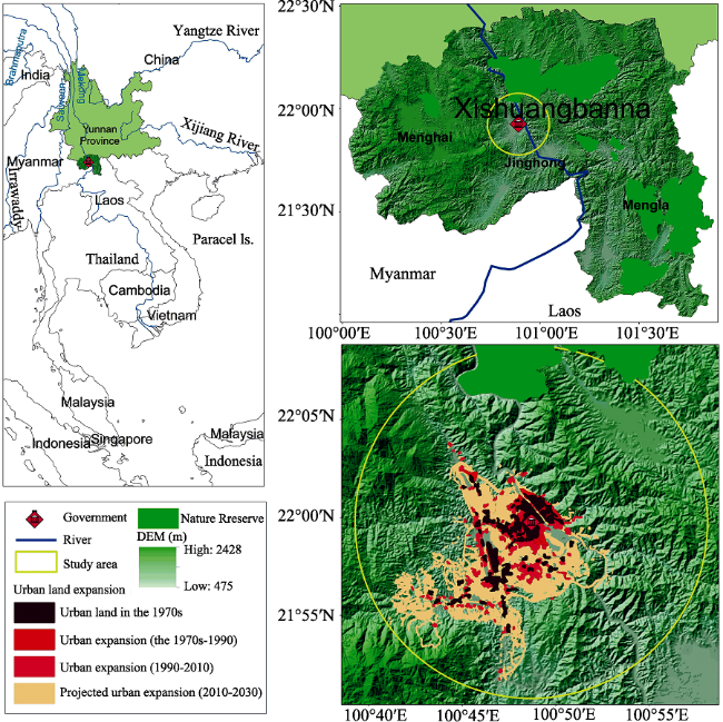
Figure 1 Location of Jinghong County and its urban land expansion during three periods
Table 1 The socio-economic development of Jinghong County from 1970 to 2010
Year GDP
(thousand $)
AOV
(%)
TI
(%)
UP
(%)
1970 0.074 46.98 30.28 11.27
1990 0.26 59.83 27.48 22.76
2010 2.11 25.34 42.71 40.57
Jinghong County includes the center of Jinghong and part of Gasa town (Cao et al., 2017). It was treated as the study case, and a circle of radius 16.5 km from the city center was drawn to cover the entire urban land of Jinghong (Figure 1).

2.2 Methods

The method flow chart contains four main steps (Figure 2a): analyses of the uncertainties of the PANDORA model, variations of urban land and BESV, the effects of urban expansion on the BESV, and the potential effect of projected urban expansion on the BESV.
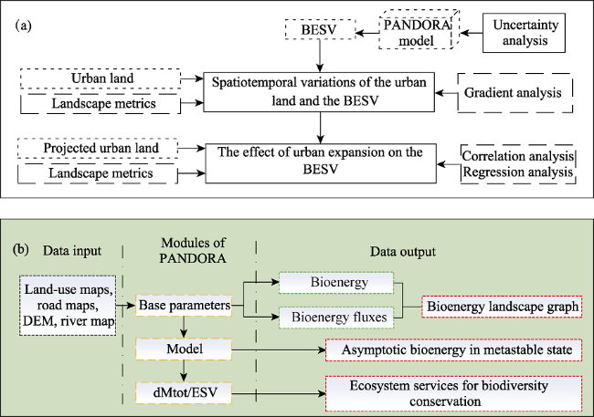
Figure 2 Schematic framework of the study (a) and the framework of the PANDORA model (b) (Pelorosso et al., 2017). BESV represents the ES for biodiversity conservation. The full line represents the steps of the study, the dashed line represents the indexes and methods used in this study, and the dotted line represents the original data and the implementation of PANDORA model.
2.2.1 Data input
Historical urban land maps were interpreted from a series of Landsat TM/ETM+ imagery (http://glovis.usgs.gov). One MSS image (Path/Row: 139/44, 139/45, 140/44, and 140/45) and two TM images (130/44 and 130/45) were acquired for the urban land map in 1976, 1990 and 2010, respectively. Supervised classification, a technique frequently used for the quantitative analysis of remote sensing image data, was applied to classify the images; the maximum likelihood algorithm was also used. Eight land use types were classified as forest, urban land, water, wetland, open space (bare land), plantation, scrub, and arable land. The visual modification was used to improve the accuracy of classification. For each map, we created 500 stratified random samples to check the accuracy. Overall accuracies of the classified maps were 85% or higher. The urban land map of 2030 was obtained by digitizing a detailed urban planning map of Jinghong, provided by the Housing and Construction Department of Yunnan Province.
Road data were digitized from the transportation map of Yunnan Province (Fu et al., 2010a). We divided the roads into three levels. The first, second, and third level roads were expressways and state roads, roads between cities and counties, and small roads between towns and villages, respectively. Digital elevation model (DEM) was derived from the National Geomatics Center of China with 25 m resolution (Yi et al., 2014a). Soil map was digitized using 1:500,000 soil maps of Yunnan Province (Wang et al., 1982).
2.2.2 PANDORA model
THEORETICAL ASSUMPTION: the model assumes that the ecosystem exchanges energy to achieve the low entropy metastable state (Kleidon et al., 2010; Vallino, 2011). Solar energy is fed into the ecosystems, which release energy through vegetative metabolism, i.e., bioenergy (Brunsell et al., 2011). Within the ecosystems, bioenergy can flow between sub-ecosystems (landscape units) and within a sub-ecosystem (between patches). The division of sub-ecosystem/landscape units depends on the distribution of barriers. In accordance with the blocking effect from large to small, the barriers are urban (0.75), roads (0.5), hills (< 700 m) to mountain (> 700 m) zones change (0.16), and rivers (0.01), respectively (Gobattoni et al., 2011). The metastable state is obtained by iterative computation. The number of iterations is determined by a balance between the logical growth of bioenergy and the reduction of bioenergy due to barriers. When the metastable state is reached, the patch with high bioenergy has a higher capacity for energy flow, and its contribution to the landscape connectivity is greater. The PANDORA model accounts for the BESV based on the unit value-based approach and weighted by the contribution to connectivity.
Variables and functions: the BESV of the jth patch belonging to the kth land use type is calculated as:
$$\text{BES}{{\text{V}}_{kj}}=V{{C}_{k}}\times \left( 1+\frac{dMto{{t}_{kj}}}{dMto{{t}_{\max }}} \right)\times {{A}_{j}} \ \ \ \ \ (1)$$
$$dMto{{t}_{kj}}=\left( \frac{Mtot_{j}^{as}-Mtot{{_{j}^{as}}^{\prime }}}{Mtot_{j}^{as}} \right)\times 100\% \ \ \ \ \ (2) $$
where VCk is the value coefficient for the kth land use type according to the modified coefficient used by Ng et al. (2013) in China; Aj is the area of the jth patch. dMtotkj represents the contribution of the jth patch with the kth land use type in the maintenance of overall system connectivity, and the patch with a higher dMtotkj value has a greater contribution to connectivity. The formula of dMtotkj calculates the change in the overall connectivity before (Mtotjas, the asymptotic bioenergy of the overall system in the metastable state) and after (Mtotjas’) changing the jth patch into an area with zero bioenergy; dMtotmax represents the maximum value of dMtot among all landscape patches and ignores the difference between land use types.
The asymptotic bioenergy of the overall system in the metastable state $(M_{_{tot}}^{as})$ can be calculated as follows:
$$M_{tot}^{as}=\sum\limits_{i=1}^{n}{M_{i}^{as}}\ \ \ \ \ (3)$$
$$M_{i}^{as}=\left( \sum\limits_{j=1}^{{{m}_{i}}}{B_{ji}^{as}\times 6.5\times {{s}_{ji}}} \right)\times (1+{{K}_{i}})\ \ \ \ \ (4)$$
where Mias represents the asymptotic bioenergy of the ith landscape unit in the metastable state; Bji represents the standardized BTC (Biological Territorial Capacity, which represents the ecosystem metabolism and is connected to land use types) of the jth patch belonging to the ith landscape unit (Ingegnoli 2011); sji represents the area of the jth patch of ith landscape unit; K is a dimensionless quantity that depends on four parameters, Kec, Khu, Kse, and Ksoil, with each parameter defined within the range of 0-1 and associated with characteristics of patch ecotones, climate, solar exposition, and soil property of each landscape unit, respectively.
Framework: the framework of the PANDORA model was shown in Figure 2b. The model contains three modules, “Base parameters,” “Model,” and “dMtot/BESV.” The operation of the first module (Base parameters) requires all data to be entered, contains land use maps, the landscape unit map, the barrier penetration, and the K value of each landscape unit. The second module, “Model,” could simulate the final metastable state. The third module, “dMtot/BESV,” could output the BESV of each patch. The PANDORA model was released on the QGIS plugin platform as an open-source plugin (https://plugins.qgis.org/plugins/pandora/).
2.2.3 Validation and uncertainty analysis of the PANDORA model
The efficiency of the PANDORA model is performed primarily in two steps: validation and uncertainty analysis.
Validation: because few studies have evaluated the BESV in the study area and there is a lack of validation data, we adopted two other ES models to assess the PANDORA BESV. One is the unit value-based approach and the other the carbon storage of the InVEST model. These two methods are also widely used in the ES assessment (Jiang 2017; Ochoa et al., 2017).
The calculation of the unit value-based approach is as follows:
$$\text{BES}{{\text{V}}_{kj}}=V{{C}_{k}}\times {{A}_{j}}\ \ \ \ \ (5)$$
where VCk is the value coefficient for the kth land use type. The value of VC of the unit value-based approach is consistent with that of the PANDORA model. Aj is the area of the jth patch.
The carbon storage data based on the InVEST model were acquired from Liu et al. (2017). In this model, the carbon storage contains four “carbon pools” in terrestrial ecosystems, i.e., soil, belowground biomass, dead organic matter, and aboveground biomass. The related data for the parameterization were collected from previous vegetation research in this area (Chen et al., 2002; Lv et al., 2007; Song et al., 2010; Liu et al., 2017).
Uncertainty analysis: the landscape connectivity of the PANDORA model refers to the flow of bioenergy. This flow is determined by the intrinsic land use types and barriers of bioenergy. The identification of the barriers is accomplished manually, and there may be human errors. To better understand how the barriers affect the results of the model, we designed four scenarios as follows: Scenario 1 is the original sample, Scenario 2 reduces the barriers (roads), Scenario 3 adds barriers (roads), and Scenario 4 increases the local fragmentation. Details are shown in Figure 4.
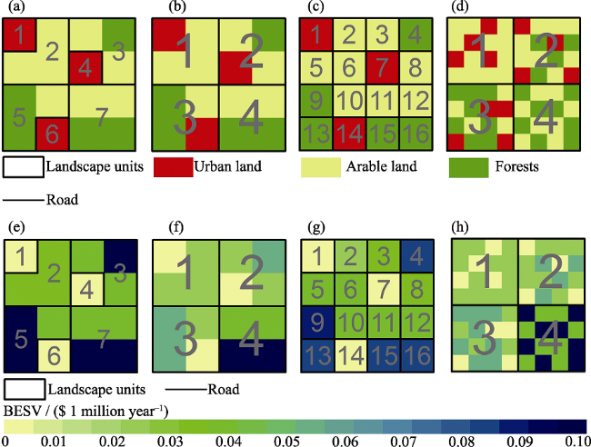
Figure 4 The uncertainty analysis of the PANDORA model. a, b, c, and d represent the Scenario 1 (the original sample), Scenario 2 (reduces roads based on the original sample), Scenario 3 (adds roads based on the original sample), and Scenario 4 (increases the local fragmentation based on the original sample), respectively. e, f, g, and h represent the BESV of Scenario 1, the BESV of Scenario 2, the BESV of Scenario 3, and the BESV of Scenario 4, respectively.
2.2.4 Indexes used and analytical methods
This study applied multiple indexes to characterize spatiotemporal variations and landscape pattern changes. Indexes used to characterize the former were annual change velocity (ACV), annual change intensity (ACI), Shannon’s entropy, and landscape expansion index (LEI). Eight landscape pattern metrics were used to characterize the composition and configuration of the landscape. Calculations and explanations of all indexes are listed in Table 2.
Table 2 Indexes of analyses of landscape changes and the BESV variation
ACV and ACI were used to depict the total change in urban land area and the BESV; Shannon’s entropy, LEI, and the standard deviational ellipse were used to demonstrate the change of urban land pattern for the whole region.
For this study, we applied class-level landscape pattern metrics (Table 1), since at this level they can provide specific information about variations of landscape patterns at the local level (Estoque et al., 2013; Estoque et al., 2016). The selection of metrics was based on previous works on urban expansion (Su et al., 2012; Estoque et al., 2013; Liu et al., 2014b; Su et al., 2014a; Su et al., 2014b; Estoque et al., 2016; Cao et al., 2017; Li et al., 2017; Liu et al., 2017). All metrics (Table 2) were obtained using Fragstats 4.2 by moving the window strategy. The calculation of metrics involved an ambiguous parameter, i.e., the size of the moving window. The width of the window was set from 200 m to 1,000 m in studies involving the urban effective influence range (Estoque et al., 2013; Estoque et al., 2016; Subasinghe et al., 2016; Cao et al., 2017). In studies involving biodiversity analysis, the window width ranged from 25 m to hundreds of meters (Angel et al., 2005; Angel et al., 2007). Based on these studies, we set up three sizes of the moving window, i.e., circles with an area of 0.1 km2, 1 km2, and 5 km2, respectively. The corresponding radius was 0.18 km, 0.56 km, and 1.26 km, respectively.

3 Results

3.1 Validation and uncertainty analysis of the PANDORA model

Figure 3 shows that, although three models had similar BESV patterns, there were differences in distributions of BESVs evaluated by PANDORA with the land use map, especially for northern forests and southern plantations. Only limited parts of the northern forests showed the higher BESV while most of the southern plantations showed the same. Results of the unit value-based approach were similar to the land use map.
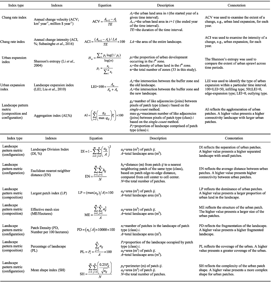
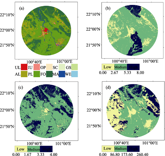
Figure 3 Land use map of the study area in 2010 (a), and the comparison of the performance of the PANDORA model (b), a unit value-based approach (c), and the InVEST model to evaluate the BESV (d). UL, IU, OP, SC, AV, AL, PL, FO, WA, and WE separately represent urban fabric, industrial units, open spaces, scrub, green space, arable land, plantation, forests, inland water, and inland wetland. b, c, and d represent the BESVs evaluated by PANDORA model ($·m-2 year-1), by the unit value-based approach (Costanza et al., 1997a; Ng et al., 2013) ($·m-2 year-1), and the carbon storage evaluated by the InVEST model (mg ha-1) in 2010, respectively. The classification of low, medium and high level applies the equal interval method.
The service values of forest and water were the highest, followed by the plantation and arable land, and the BESVs of the urban and industrial area were the lowest. The carbon storage of the InVEST model was also similar to the unit value-based approach. However, BESV of InVEST was slightly different from that of the unit value-based approach, since the carbon storage of arable land was low. Therefore, it is clear that the distribution of different land use types affected the BESVs across three models, and the PANDORA model is more robust considering the connectivity of certain land use.
We designed four scenarios to assistant barrier effects on BESV simulations in PANDORA. The total BESV of Scenario 1 was the highest, followed by Scenario 3, and Scenarios 2 and 4 were the lowest. The overall BESV in Scenarios 2 and 4 were comparable. Differences between Scenarios 1 and 3 reveal that the increase in roads would reduce the BESV. The existence of urban land within a landscape unit would reduce the BESV unit revealed by comparisons of Scenarios 1, 2, and 3. The decreasing effect was higher than increasing the road effect. By comparing Scenarios 2 and 4, the PANDORA model was found to be insensitive to changes in the fragmentation within a landscape unit.

3.2 Spatiotemporal variation of urban land and the BESV

3.2.1 Total change in urban land area and the region’s BESV
The urban land expanded from 18.64 km2 in the 1970s to 36.81 km2 in 2010. The expansion was in patterns of ‘sprawling’ (Figure 5a). The regional BESV decreased gradually, with a 9% decrease in total. Also, the corresponding ACV and ACI of urban expansion increased from 0.21 km2 year-1 and 0.02% to 0.76 km2 year-1 and 0.08%, respectively (Figure 5b).
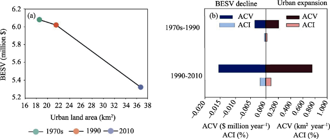
Figure 5 Annual variation of both urban land and the region’s BESV. ACV and ACI represent annual change velocity and annual change intensity, respectively.
Shannon’s entropy of the urban land increased from 0.61 to 0.68. The regional BESV decreased from $ 6.08 million year-1 to $ 5.32 million year-1. Its ACV and ACI decreased from -0.0035 $ million year-1 to -0.0153 $ million year-1 and from -0.0004% to and -0.0018%, respectively. Also, changes in both urban land and the BESV during 1990-2010 (Period 2) were larger than during the 1970s-1990 (Period 1).
3.2.2 The change of urban land pattern in the region
The transformation of land use in Period 1 was not noticeable; the Fuzzy Kappa Index between land use maps of the 1970s and 1990 was 0.96, which indicated that their landscape patterns were close. The Fuzzy Kappa Index between land use maps of 1990 and 2010 in Period 2 was just 0.18, indicating the dramatic change in land use.
Shannon’s entropy of urban land in Period 2 was only 1.1 times that of Period 1. The expansion center and range of the whole urban land had a low deviation (Figure 6a). The newly grown urban land showed a different pattern between two periods (Figure 6b). In Period 1, the urban land expanded along the NW-SE, and the expansion type was edge-expansion (69%) and filling (31%). In the last 20 years, the urban land expanded rapidly, and the outlying expansion type increased to 18%.
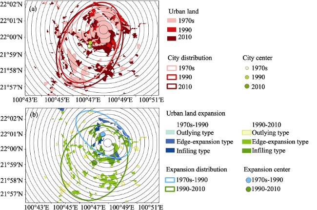
Figure 6 Distributions of urban land and its expansion from the 1970s to 2010 (a. The distribution of urban land; b. The distribution of the newly grown urban land)
3.2.3 The urban expansion and BESV changes along a distance-gradient
Three typical relationships exist between urban expansion and BESV variations along with the distance from city center (Figure 7). Relationship (I) appeared within 6 km, in which urban expansion and BESV variations were both apparent. Relationship (II) appeared from 4 to 8 km, in which the urban land expanded slightly and always accompanied by the BESV increase. Relationship (III) appeared further than 8 km, in which the urban land expanded slightly and the BESV clearly decreased. The urban expansion and the BESV variation of Period 2 were in a higher degree than Period 1 (Figure 7).
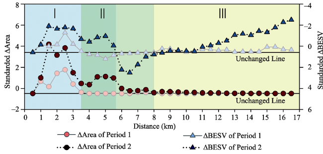
Figure 7 The distance gradients for the difference between urban land areas (∆Area) and the difference between BESVs (∆BESV) in different periods. The left longitudinal axis shows the standardized ∆Area, and its value increases from bottom to top along the axis. The right longitudinal axis shows the standardized ∆BESV, and its value decreases from bottom to top. The 0 in the X-axis represents the city center. Because of the normalization, the plus-minus state in the Figure is not the same as those in the raw data while the fluctuated trends of these data were consistent with those of the raw data.

3.3 The effect of urban expansion on BESV

3.3.1 The effect of urban landscape pattern changes on BESV
Variation of BESVs was highly related to urban landscape pattern changes, and their relationship strengthened with a decrease in the moving window size (Table 3). In both Periods 1 and 2, the ∆ of all selected landscape metrics was significantly correlated with its corresponding ∆BESV (p<0.01). Overall, the landscape metrics representing the landscape composition (∆LP, ∆ME, and ∆PL) were negatively correlated with ∆BESVs, while metrics that represent the landscape configuration (∆DI, ∆EN, ∆PD, and ∆SH) were positive.
Table 3 Pearson correlation coefficients between the difference (∆) of BESVs and the difference (∆) of landscape metrics
Period Moving-window size/km2 ∆AI ∆DI ∆EN ∆LP ∆ME ∆PD ∆PL ∆SH
∆BESV
(1970s-1990)
0.1 -0.13 0.35 0.14 -0.65 -0.62 0.14 -0.65 0.15
1 0.10 0.22 0.06 -0.43 -0.40 0.19 -0.42 0.20
5 0.09 0.12 0.02 -0.21 -0.21 0.11 -0.26 0.15
∆BESV
(1990-2010)
0.1 -0.16 0.19 0.14 -0.55 -0.45 0.08 -0.55 -0.01
1 0.07 0.14 0.10 -0.31 -0.24 0.10 -0.30 0.07
5 0.01 0.04 0.03 -0.18 -0.14 0.06 -0.16 0.04
The absolute value of correlation coefficients between ∆landscape composition indexes and ∆BESVs was often higher than the coefficients between ∆landscape configuration indexes and ∆BESVs. ∆AI showed a negative correlation with ∆BESV at 0.1 km2 of the moving-window, while any such correlation between them became positive as the size of the moving-window increased to 0.56 km2. In addition, if the size of the moving-window was set to a minimum (such as 0.1 km2), the correlation coefficients of most metrics showed their highest value. Consequently, we used 0.1 km2 as the appropriate size of the moving-window for the subsequent analyses.
The correlations between ∆landscape metrics and the corresponding ∆BESVs are all significant (0.01 significant level). AI aggregation index; DI landscape division index; EN Euclidean nearest neighbor distance; LP largest patch index; ME effective mesh size; PD patch density; PL percentage of landscape; SH area-weighted mean shape index.
3.3.2 The potential effect of future urban planning on BESV
Considering the apparent difference between urban expansion in Periods 1 and 2, regression models between ∆BESV and ∆landscape metrics of these two periods were constructed separately. ∆AI, ∆DI, ∆LP, ∆SH, and ∆PL were added to the regression model of Period 1, while ∆PL was replaced by ∆ME in Period 2 (Table 4).
Table 4 The stepwise regression analysis for the difference (∆) of BESVs and the difference (∆) of landscape metrics
Period R2 p Regression model
1970s-1990 0.480 <0.001 ∆BESV=0.053+0.005∆AI-1.624∆DI-0.038∆LP-0.019∆PL+1.552∆SH
1990-2010 0.327 <0.001 ∆BESV=0.001+0.003∆AI-0.902∆DI-0.063∆LP+0.226∆ME+0.890∆SH
Based on the regional urban planning map, the study area’s urban land will grow significantly until 2030, reaching 91.04 km2 by that year. The ACV and ACI will reach about 2.71 km2 year-1 and 0.32%, respectively. The Shannon’s entropy will also rise to 0.82, presenting urban land that is significantly fragmented.
In these projected urban patches, the outlying type will increase to 22%, while the infilling type will fall to 7%. Overall, the projected urban landscape pattern is similar to the urban landscape in 2010, both of them sprawling rapidly. Hence, we applied the model of Period 2 in Table 4 to predict the potential changes in BESV in the projected urban land.
Hence, 95% of the projected urban land shows a decreasing trend of BESV, while 5% of the area shows an increasing trend (Figure 8). In areas with decreasing BESV, the BESV of 51% of the area will decrease by $2-3 m-2 year-1, 26% of the area will decline by $1-2 m-2 year-1, and the remaining areas will lose less BESV.
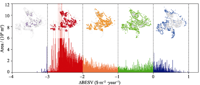
Figure 8 Statistics of BESV changes (∆BESV) of projected urban land in 2030. Different colors represent the different range of variations in BESV. The small figure with different colors above represents the spatial distribution that the color represents below.
Although the increment of the BESV will be limited, ranging from $0 to $1 m-2 year-1, the BESV of the projected urban land closest to the existing urban land will fall significantly, decreasing as the distance from it increases. Further, BESV of the area on the fringe of projected urban land is predicted to have an upward trend.

4 Discussion

4.1 Validation and uncertainty analysis of the PANDORA model

Generally, the results derived by PANDORA were consistent with the two referenced models (Figure 3). The similarity is mainly because all the models were highly affected by the distribution of land use types. In Figure 3b, the distribution of BESVs in the south and north indicate that the PANDORA model was also affected by the distribution of the bioenergy barriers; and Figure 4 shows that the existence of urban land might negatively affect the evaluation of BESV. The PANDORA had a weak ability to identify the fragmentation changes within a landscape unit.
The impact of urban land on BESV might be reflected in the following ways: (1) because urban land cannot provide the BESV, its existence would reduce the bioenergy of the whole landscape; and (2) the barrier effect level of urban land was set to maximum in the PANDORA model. Thus, the barrier of urban land had a more obvious effect on bioenergy reduction.
Since the bioenergy reduction transformed the bioenergy of the landscape unit to a lower metastable state, the total BESV of the unit became correspondingly lower. Comparisons over Scenarios 1, 2 and 3 indicate that the existence of urban land was more effective than the increase of road barriers to the BESV reduction. Also, the comparison between Scenarios 2 and 4 show that the dispersed urban and compact urban land had similar effects on the reduction of BESV. Therefore, when using the PANDORA model to estimate BESV, the urban land should be divided into as few landscape units as possible.
We also found PANDORA was insensitive to urban landscape fragmentation changes within landscape units revealed by Scenarios 2 and 4. Although the effect of fragmentation on ecosystem services has both positive and negative effects (Mitchell et al., 2015), the fragmentation associated with barriers in PANDORA negatively affected the bioenergy flow between landscape units (Gobattoni et al.). Hence, the fragmentation effect by roads could be revealed during model calculation while the effect of urban fragmentation within the landscape unit on BESV could not be manifested.

4.2 Spatiotemporal variations of urban land and BESV

Figures 5 and 6 indicate that changes in the urban land pattern were more evident in the newly grown urban land than reflecting urban land as a whole. Overall, the changes of the whole regional BESV were closely related to the increment of urban land. The rapid rate of urban expansion was also implied in previous studies of this region (Cao et al., 2017). Furthermore, our results were consistent with previous findings that the BESV decreased as a consequence of dramatic changes in land use in the study region (Liu et al., 2017; Smajgl et al., 2015). The increased urban land was chiefly transformed from arable land, plantation, and shrub (Cao et al., 2017). Further, arable land and plantation expanded into natural vegetation to replenish losses (Fu et al., 2010b; Li et al., 2008). Such changes in land use type lead to a reduced BESV.
We classified the city into three parts - hinterland, periphery, and nonurban - (Benza et al., 2016; Wu et al., 2015) in which the three relationships in Figure 7 occurred, so that the BESV of the hinterland and nonurban land decreased significantly, while the BESV of the periphery increased equally significantly. The BESV variations along the urban-nonurban gradient coincided with the results of most previous studies (Benza et al., 2016; Kroll et al., 2012; Radford et al., 2013; Wu et al., 2015; Zhou et al., 2011).
The fluctuation of the BESV along with the gradient was chiefly related to net land use changes. In the inner city, the net land use change was primarily manifested by the encroachment of urban land onto arable land (Cao et al., 2017; Fu et al., 2010b; Li et al., 2008). Since the 1970s, arable land along the city’s periphery was gradually replaced by plantations (Cao et al., 2017), the BESV of which was higher than that of arable land. Thus, the increased plantation in the outer city contributed to the increased BESV. Although the peripheral BESV increase might be related to increased cover of green lands in urban fringes (Radford et al., 2013), the BESV change in the nonurban land was caused primarily by changes in arable land and plantation.

4.3 The effect of urban expansion on BESV

The results show that the correlation between ΔBESV and Δlandscape metrics decreases with the increasing moving-window size. In our study, the changes of all selected metrics were significantly correlated with ΔBESV and complied with several previous studies (Cai et al., 2016; Liu et al., 2017; Su et al., 2012). Further, the correlation between the Δlandscape composition indexes and ΔBESVs is higher than that between Δlandscape structure indexes and ΔBESVs. Such a result was consistent with the effect of landscape pattern change on biodiversity (Eigenbrod, 2016).
Because in this study we introduced the urban class instead of all classes into the models in Cai et al., 2016, the contribution of landscape metrics to the BESV change (Table 4) was lower relatively than in previous studies (Cai et al., 2016). Moreover, the effect of land use changes on the BESVs differed among land use types (Kindu et al., 2016).
During two-time intervals, AI, DI, LP, and SH were all inputted into the model of ΔBESV and Δlandscape metrics, while PL and ME were inputted into the model only during Periods 1 and 2, respectively. These metrics represented three landscape aspects: AI and DI indicated the fragmentation; AI, ME, LP, and PL represented the proportion of urban land, and SH presented the complexity of urban patch shape. Therefore, we attributed changes of BESVs in grains to the net urban expansion (landscape composition changes) and landscape configuration changes.
The development of Chinese cities is regulated by government policies. The government’s urban planning map was involved in simulating future urban land. We applied changes in landscape patterns to predict the potential changes in the BESV due to projected urban expansion. The prediction model shows that the fragmentation, the proportion of urban patches, and the complexity of urban patch shape would affect the effect of urban expansion on the BESV.
The inference of fragmentation in the prediction model differed with the result of correlation analysis, which was due to the suppression effect of the multiple regression analysis (Friedman et al., 2005; Lipovetsky et al., 2004; Mayer et al., 2016). Although the relationship between the independent and dependent variables in the multiple regression analysis was controlled by other variables, it was normal that the result of correlation analysis was inconsistent with that of regression analysis. Considering the inevitability of urban expansion, we could change only the landscape fragmentation and the complexity of urban patch shape to ameliorate the BESV in the region.
The compact urban clusters were conducive for maintaining the BESV, and the higher complexity of urban patches also facilitated its support. Considering these two factors, we suggest that the urban land in our study should be built as a compact, high-density residential area. This will further improve the utilization of existing infrastructures and reduce related external costs due to urban expansion (Estoque et al., 2016; Gagné et al., 2010). However, a dense urban pattern is not consistent with the planning development theme of Jinghong, which is designed as a tourist attraction. The high-density pattern will lead to an increase in traffic congestion and to crowded services (Estoque et al., 2016).
The effects of urban expansion on ecosystem services are still uncertain. Although the direction or magnitude of urban land changes differs between cities, most of the available cases are locally specific. Because ecosystem services occur in bundles rather than in isolated landscapes, our cases focus on one of the several ecosystem services to explain its general response to land use changes. We tried, as a result, to construct a framework to optimize urban planning for biodiversity conservation and apply it to a biodiversity hotspot.

5 Conclusions

Using the PANDORA model, we determined BESV for both land use types and landscape connectivity, which enables it to establish the relationship between the BESV variation and urban expansion from the perspectives of landscape composition and landscape configuration. Over the last 40 years, we see in Xishuangbanna an accelerated trend of the reducing rate of the BESV, which, as of 2010, has decreased to $5.32 million year-1 with an annual loss of $0.02 million. Our results show that both landscape composition and landscape configuration can affect the regional BESV and that the improvement of the landscape configuration is closely associated with regulating the urban land expansion rate. We believe that although the compact urban land with complexity patch shape could spare land and prevent a reduced BESV, such urban patterns reduce the city’s social services quality. Future work in urban planning should focus on a trade-off between compact and landscape sprawl, so important for maintaining the regional BESV.

The authors have declared that no competing interests exist.

1
Angel S, Parent J, Civco D, 2007. Urban sprawl metrics: An analysis of global urban expansion using GIS. Tampa, Florida: ASPRS 2007 Annual Conference.

2
Angel S, Sheppard S C, Civco D L et al., 2005. The Dynamics of Global Urban Expansion. Washington DC: World Bank.

3
Benza M, Weeks J R, Stow D A et al., 2016. A pattern-based definition of urban context using remote sensing and GIS. Remote Sensing of Environment, 183: 250-264.

4
Brunsell N A, Schymanski S J, Kleidon A, 2011. Quantifying the thermodynamic entropy budget of the land surface: Is this useful? Earth System Dynamics, 2(26): 87-103.

DOI

5
Cai Y B, Li H M, Ye X Y et al., 2016. Analyzing three-decadal patterns of land use/land cover change and regional ecosystem services at the landscape level: Case study of two coastal metropolitan regions, eastern China. Sustainability, 8(8): 773.

6
Cao H, Liu J, Fu C et al., 2017. Urban expansion and its impact on the land use pattern in Xishuangbanna since the reform and opening up of China. Remote Sensing, 9(2): 137.

7
Cao M, Zhang J H, 1997. Tree species diversity of tropical forest vegetation in Xishuangbanna, SW China. Biodiversity & Conservation, 6(7): 995-1006.

8
Chen H W, Feng X, Liu Y G et al., 2002. Study of biomass of six kinds of plantations in Xishuangbanna. Yunan Forestry Science & Technology, 3: 19-22.

9
Costanza R, d'Arge R, de Groot R et al., 1997. The value of the world’s ecosystem services and natural capital. Nature, 387: 253-260.

10
De Montis A, Caschili S, Mulas M et al., 2016. Urban-rural ecological networks for landscape planning. Land Use Policy, 50: 312-327.

11
Eigenbrod F, 2016. Redefining landscape structure for ecosystem services. Current Landscape Ecology Reports, 1(2): 80-86.

DOI

12
Estoque R C, Murayama Y, 2013. Landscape pattern and ecosystem service value changes: Implications for environmental sustainability planning for the rapidly urbanizing summer capital of the Philippines. Landscape and Urban Planning, 116: 60-72.

DOI

13
Estoque R C, Murayama Y, 2016. Quantifying landscape pattern and ecosystem service value changes in four rapidly urbanizing hill stations of Southeast Asia. Landscape Ecology, 31(7): 1481-1507.

DOI

14
Friedman L, Wall M, 2005. Graphical views of suppression and multicollinearity in multiple linear regression. American Statistician, 59(2): 127-136.

DOI

15
Fu W, Liu S L, DeGloria S D et al., 2010a. Characterizing the “fragmentation-barrier” effect of road networks on landscape connectivity: A case study in Xishuangbanna, Southwest China. Landscape and Urban Planning, 95(3): 122-129.

16
Fu Y, Chen J, Guo H, et al. 2010b. Agrobiodiversity loss and livelihood vulnerability as a consequence of converting from subsistence farming systems to commercial plantation-dominated systems in Xishuangbanna, Yunnan, China: A household level analysis. Land Degradation & Development, 21(3): 274-284.

17
Gagné S A, Fahrig L, 2010. The trade-off between housing density and sprawl area: Minimising impacts to forest breeding birds. Basic and Applied Ecology, 11(8): 723-733.

DOI

18
Gobattoni F, Pelorosso R, Lauro G et al., 2011. A procedure for mathematical analysis of landscape evolution and equilibrium scenarios assessment. Landscape and Urban Planning, 103(3/4): 289-302.

19
Ingegnoli V, 2011. Non-Equilibrium Thermodynamics, Landscape Ecology and Vegetation Science. Rijeka: InTech.

20
Jiang W, 2017. Ecosystem services research in China: A critical review. Ecosystem Services, 26(Part A): 10-16.

DOI

21
Kindu M, Schneider T, Teketay D et al., 2016. Changes of ecosystem service values in response to land use/land cover dynamics in Munessa-Shashemene landscape of the Ethiopian highlands. Science of the Total Environment, 547: 137-147.

22
Kleidon A, Malhi Y, Cox P M, 2010. Introduction: Maximum entropy production in environmental and ecological systems. Philosophical Transactions of the Royal Society of London, 365(1545): 1297-1302.

DOI

23
Kroll F, Müller F, Haase D et al., 2012. Rural-urban gradient analysis of ecosystem services supply and demand dynamics. Land Use Policy, 29(3): 521-535.

24
Lawler J J, Lewis D J, Nelson E et al., 2014. Projected land-use change impacts on ecosystem services in the United States. Proceedings of the National Academy of Sciences of the United States of America, 111(20): 7492-7497.

25
Li H, Ma Y, Aide T M et al., 2008. Past, present and future land-use in Xishuangbanna, China and the implications for carbon dynamics. Forest Ecology and Management, 255(1): 16-24.

26
Li H L, Peng Jian, Liu Y X et al., 2017. Urbanization impact on landscape patterns in Beijing City, China: A spatial heterogeneity perspective. Ecological Indicators, 82: 50-60.

27
Li X, Yeh A G-O, 2004. Analyzing spatial restructuring of land use patterns in a fast growing region using remote sensing and GIS. Landscape and Urban Planning, 69(4): 335-354.

DOI

28
Lipovetsky S, Conklin W M, 2004. Enhance-synergism and suppression effects in multiple regression. International Journal of Mathematical Education in Science and Technology, 35(3): 391-402.

DOI

29
Liu S L, Deng L, Zhao Q H et al., 2011. Effects of road network on vegetation pattern in Xishuangbanna, Yunnan Province, Southwest China. Transportation Research Part D Transport & Environment, 16(8): 591-594.

30
Liu S L, Deng L, Dong S K et al., 2014a. Landscape connectivity dynamics based on network analysis in the Xishuangbanna Nature Reserve, China. Acta Oecologica, 55: 66-77.

31
Liu S L, Dong Y H, Deng L et al., 2014b. Forest fragmentation and landscape connectivity change associated with road network extension and city expansion: A case study in the Lancang River Valley. Ecological Indicators, 36(36): 160-168.

32
Liu S L, Yin Y J, Liu X H et al., 2017. Ecosystem Services and landscape change associated with plantation expansion in a tropical rainforest region of Southwest China. Ecological Modelling, 353: 129-138.

33
Liu W J, Hu H B, Ma Y X et al., 2006. Environmental and socioeconomic impacts of increasing rubber plantations in Menglun Township, Southwest China. Mountain Research & Development, 26(3): 245-253.

34
Lv X H, Han Y P, Luo Y, 2007. Observation on 58 cases of threatened miscarriage. Journal of Yunnan Chinese Medicine, 28(12): 11.

35
Mayer A L, Buma B, Davis A et al., 2016. How landscape ecology informs global land-change science and policy. Bioscience, 66(6): 458-469.

36
Mitchell M G E, Suarez-Castro A F, Martinez-Harms M et al., 2015. Reframing landscape fragmentation's effects on ecosystem services. Trends in Ecology & Evolution, 30(4): 190-198.

37
Ng C N, Xie Y J, Yu X J, 2013. Integrating landscape connectivity into the evaluation of ecosystem services for biodiversity conservation and its implications for landscape planning. Applied Geography, 42: 1-12.

DOI

38
Ochoa V, Urbina-Cardona N, 2017. Tools for spatially modeling ecosystem services: Publication trends, conceptual reflections and future challenges. Ecosystem Services, 26(Part A): 155-169.

DOI

39
Pelorosso R, Gobattoni F, Geri F et al., 2016. Evaluation of ecosystem services related to bio-energy landscape connectivity (BELC) for land use decision making across different planning scales. Ecological Indicators, 61(Part 1): 114-129.

40
Pelorosso R, Gobattoni F, Geri F et al., 2017. PANDORA 3.0 plugin: A new biodiversity ecosystem service assessment tool for urban green infrastructure connectivity planning. Ecosystem Services, 26(Part B): 476-482.

41
Peng J, Liu Z C, Liu Y X et al., 2015. Multifunctionality assessment of urban agriculture in Beijing City, China. Science of the Total Environment, 534: 343-351.

42
Radford K G, James P, 2013. Changes in the value of ecosystem services along a rural-urban gradient: A case study of Greater Manchester, UK. Landscape and Urban Planning, 109: 117-127.

DOI

43
Shen Z H, Zhang Z M, Hu J M et al., 2016. Protection and utilization of plant biodiversity resources in dry valleys of Southwest China. Biodiversity Science, 24(4): 475-488.

44
Smajgl A, Xu J C, Egan S et al., 2015. Assessing the effectiveness of payments for ecosystem services for diversifying rubber in Yunnan, China. Environmental Modelling & Software, 69(Suppl.C): 187-195.

45
Song Q H, Zhang Y P, 2010. Biomass, carbon sequestration and its potential of rubber plantations in Xishuangbanna, Southwest China. Chinese Journal of Ecology, 29(10): 1887-1891.

46
Song W, Deng X Z, Yuan Y W et al., 2015. Impacts of land-use change on valued ecosystem service in rapidly urbanized North China Plain. Ecological Modelling, 318: 245-253.

47
Su S L, Hu Y N, Luo F H et al., 2014a. Farmland fragmentation due to anthropogenic activity in rapidly developing region. Agricultural Systems, 131: 87-93.

48
Su S L, Ma X Y, Xiao R, 2014b. Agricultural landscape pattern changes in response to urbanization at ecoregional scale. Ecological Indicators, 40: 10-18.

DOI

49
Su S L, Xiao R, Jiang Z L et al., 2012. Characterizing landscape pattern and ecosystem service value changes for urbanization impacts at an eco-regional scale. Applied Geography, 34: 295-305.

50
Subasinghe S, Estoque R C, Murayama Y, 2016. Spatiotemporal analysis of urban growth using GIS and remote sensing: A case study of the Colombo Metropolitan Area, Sri Lanka. ISPRS International Journal of Geo- Information, 5(11): 197.

DOI

51
Tan M H, Li X B, Xie H et al., 2005. Urban land expansion and arable land loss in China: A case study of Beijing-Tianjin-Hebei region. Land Use Policy, 22(3): 187-196.

52
Vallino J J, 2011. Differences and implications in biogeochemistry from maximizing entropy production locally versus globally. Earth System Dynamics, 2(1): 69-85.

DOI

53
Wang J Y, Zhu H Q, Yu N Z et al., 1982. Forestry soil map of Yunnan Province, China. Forest Inventory and Planning of Yunnan Province, 1: 18-25.

54
Wu W J, Zhao S Q, Zhu C et al., 2015. A comparative study of urban expansion in Beijing, Tianjin and Shijiazhuang over the past three decades. Landscape and Urban Planning, 134(Suppl. C): 93-106.

55
Xie G D, Lu C X, Leng Y F et al., 2003. Ecological assets valuation of the Tibetan Plateau. Journal of Natural Resources, 18(2): 189-196.

56
Yi K, Tani H, Li Q et al., 2014a. Mapping and evaluating the urbanization process in Northeast China using DMSP/OLS Nighttime Light Data. Sensors, 14(2): 3207-3226.

57
Yi Z F, Cannon C H, Chen J et al., 2014b. Developing indicators of economic value and biodiversity loss for rubber plantations in Xishuangbanna, Southwest China: A case study from Menglun township. Ecological Indicators, 36(1): 788-797.

58
Ying L X, Shen Z H, Chen J D et al., 2014. Spatiotemporal patterns of road network and road development priority in Three Parallel Rivers Region in Yunnan, China: An Evaluation Based on Modified Kernel Distance Estimate. Chinese Geographical Science, 24(1): 39-49.

59
Zhang J J, Fu M C, Zeng H et al., 2013. Variations in ecosystem service values and local economy in response to land use: A case study of Wu'an, China. Land Degradation & Development, 24(3): 236-249.

60
Zhou X L, Wang Y C, 2011. Spatial-temporal dynamics of urban green space in response to rapid urbanization and greening policies. Landscape and Urban Planning, 100(3): 268-277.

DOI

61
Ziegler A D, Fox J M, Xu J C, 2009. The Rubber Juggernaut. Science, 324(5930): 1024-1025.

DOI

62
Zurlini G, Petrosillo I, Jones K B et al., 2013. Highlighting order and disorder in social-ecological landscapes to foster adaptive capacity and sustainability. Landscape Ecology, 28(6): 1161-1173.

Outlines

/