
Journal of Geographical Sciences >
Effects of current climate, paleo-climate, and habitat heterogeneity in determining biogeographical patterns of evergreen broad-leaved woody plants in China
*Corresponding author: Shen Zehao, Professor, specialized in landscape ecology. E-mail: shzh@pku.edu.cn
Author: Xu Yue, PhD, Assistant Researcher, specialized in biogeography. E-mail: xuyue@caf.ac.cn
Received date: 2018-05-10
Accepted date: 2019-01-22
Online published: 2019-07-25
Supported by
National Natural Science Foundation of China, No.41790425, No.41701055
National Key R&D Program of China, No.2017YFC0505200
Major Project of the Yunnan Science and Technology Department, No.2018 FY001(-002)
Copyright
Understanding biogeographic patterns and the mechanisms underlying them has been a main issue in macroecology and biogeography, and has implications for biodiversity conservation and ecosystem sustainability. Evergreen broad-leaved woody plants (EBWPs) are important components of numerous biomes and are the main contributors to the flora south of 35°N in China. We calculated the grid cell values of species richness (SR) for a total of 6265 EBWP species in China, including its four growth-forms (i.e., tree, shrub, vine, and bamboo), and estimated their phylogenetic structure using the standardized phylogenetic diversity (SPD) and net relatedness index (NRI). Then we linked the three biogeographical patterns that were observed with each single environmental variable representing the current climate, the last glacial maximum (LGM)-present climate variability, and habitat heterogeneity, using ordinary least squares regression with a modified t-test to account for spatial autocorrelation. The partial regression method based on a general linear model was used to decompose the contributions of current and historical environmental factors to the biogeographical patterns observed. The results showed that most regions with high numbers of EBWP species and phylogenetic diversity were distributed in tropical and subtropical mountains with evergreen shrubs extending to Northeast China. Current mean annual precipitation was the best single predictor. Topographic variation and its effect on temperature variation was the best single predictor for SPD and NRI. Partial regression indicated that the current climate dominated the SR patterns of Chinese EBWPs. The effect of paleo-climate variation on SR patterns mostly overlapped with that of the current climate. In contrast, the phylogenetic structure represented by SPD and NRI was constrained by paleo-climate to much larger extents than diversity, which was reflected by the LGM-present climate variation and topography-derived habitat heterogeneity in China. Our study highlights the importance of embedding multiple dimensions of biodiversity into a temporally hierarchical framework for understanding the biogeographical patterns, and provides important baseline information for predicting shifts in plant diversity under climate change.
XU Yue , SHEN Zehao , YING Lingxiao , ZANG Runguo , JIANG Youxu . Effects of current climate, paleo-climate, and habitat heterogeneity in determining biogeographical patterns of evergreen broad-leaved woody plants in China[J]. Journal of Geographical Sciences, 2019 , 29(7) : 1142 -1158 . DOI: 10.1007/s11442-019-1650-x
Table 1 Matrix of Pearson’s correlation coefficients among the 13 environmental variables. The boldfaced value in each column indicates the most correlated variable within that column. |
| MAT | TSN | MTCQ | MAP | PSN | PDQ | MATA | MAPA | MATV | MAPV | ELER | MATR | MAPR | |
|---|---|---|---|---|---|---|---|---|---|---|---|---|---|
| MAT | 1.000 | -0.474 | 0.922 | 0.712 | -0.548 | 0.662 | -0.650 | 0.212 | -0.171 | 0.208 | -0.215 | -0.244 | 0.279 |
| TSN | -0.474 | 1.000 | -0.718 | -0.624 | 0.336 | -0.417 | 0.800 | -0.033 | 0.814 | 0.184 | -0.427 | -0.421 | -0.439 |
| MTCQ | 0.922 | -0.718 | 1.000 | 0.728 | -0.599 | 0.682 | -0.798 | 0.112 | -0.420 | 0.057 | 0.011 | -0.013 | 0.362 |
| MAP | 0.712 | -0.624 | 0.728 | 1.000 | -0.578 | 0.846 | -0.514 | 0.306 | -0.480 | -0.019 | 0.068 | 0.037 | 0.530 |
| PSN | -0.548 | 0.336 | -0.599 | -0.578 | 1.000 | -0.734 | 0.493 | -0.168 | 0.246 | 0.076 | -0.031 | 0.007 | -0.227 |
| PDQ | 0.662 | -0.417 | 0.682 | 0.846 | -0.734 | 1.000 | -0.439 | 0.292 | -0.291 | 0.050 | -0.081 | -0.112 | 0.334 |
| MATA | -0.650 | 0.800 | -0.798 | -0.514 | 0.493 | -0.439 | 1.000 | -0.113 | 0.587 | 0.066 | -0.214 | -0.193 | -0.240 |
| MAPA | 0.212 | -0.033 | 0.112 | 0.306 | -0.168 | 0.292 | -0.113 | 1.000 | -0.020 | 0.334 | -0.165 | -0.162 | 0.059 |
| MATV | -0.171 | 0.814 | -0.420 | -0.480 | 0.246 | -0.291 | 0.587 | -0.020 | 1.000 | 0.407 | -0.665 | -0.661 | -0.407 |
| MAPV | 0.208 | 0.184 | 0.057 | -0.019 | 0.076 | 0.050 | 0.066 | 0.334 | 0.407 | 1.000 | -0.512 | -0.497 | -0.242 |
| ELER | -0.215 | -0.427 | 0.011 | 0.068 | -0.031 | -0.081 | -0.214 | -0.165 | -0.665 | -0.512 | 1.000 | 0.989 | 0.481 |
| MATR | -0.244 | -0.421 | -0.013 | 0.037 | 0.007 | -0.112 | -0.193 | -0.162 | -0.661 | -0.497 | 0.989 | 1.000 | 0.444 |
| MAPR | 0.279 | -0.439 | 0.362 | 0.530 | -0.227 | 0.334 | -0.240 | 0.059 | -0.407 | -0.242 | 0.481 | 0.444 | 1.000 |
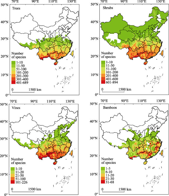
Figure 1 The spatial patterns of species richness of the four growth forms (i.e., tree, shrub, vine, and bamboo) of evergreen broad-leaved woody plants in China |
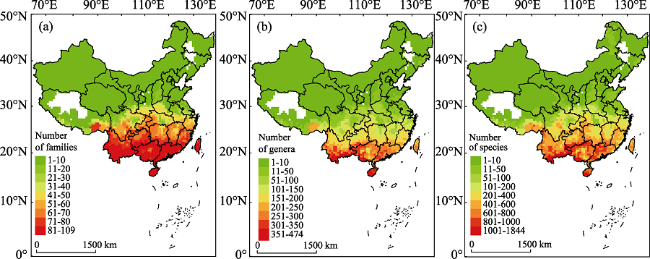
Figure 2 Distribution patterns for richness of (a) families, (b) genera, and (c) species (SR) for evergreen broadleaved woody plants (EBWPs) in China. Empty areas indicate the absence of EBWPs. |
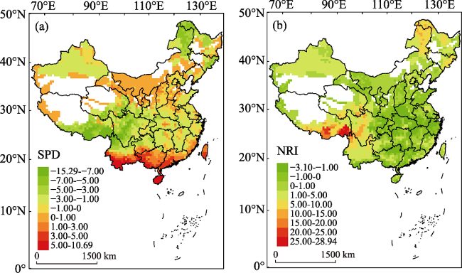
Figure 3 Spatial variation in (a) standardized phylogenetic diversity (SPD) and (b) net relatedness index (NRI). Empty areas are those with less than two species of EBWP recorded in one grid cell. |
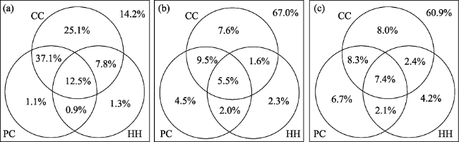
Figure 4 The partitioning of the variance (R2, %) in (a) log(SR), (b) SPD, and (c) NRI accounted for by each of the three environmental factors using partial regression methods. See Legendre and Legendre (1998) for details of the method. CC = current climate; PC = paleo-climate; HH = habitat heterogeneity. |
Table 1 The r2 of univariate OLS regression models with p values of modified t-test of the biogeographical indices against environmental variables, all with spatial autocorrelation. The minus in braces indicate negative relationship, the statistical significant p values are boldfaced. |
| Environmental factors | Predictors | SR | SPD | NRI | |||
|---|---|---|---|---|---|---|---|
| r2 | p | r2 | p | r2 | p | ||
| Current climate | MAT | 0.469 | 0.038 | 0.151 | 0.014 | (-)0.135 | 0.078 |
| MAP | 0.733 | 0.006 | (-)0.005 | 0.672 | (-)0.003 | 0.779 | |
| MTCM | 0.692 | 0.013 | 0.073 | 0.084 | (-)0.051 | 0.295 | |
| PDQ | 0.463 | 0.048 | 0.025 | 0.344 | (-)0.018 | 0.541 | |
| TSN | (-)0.561 | 0.033 | (-)0.013 | 0.537 | (-)0.078 | 0.277 | |
| PSN | (-)0.297 | 0.088 | 0.038 | 0.336 | (-)0.084 | 0.247 | |
| Paleo-climate | MATA | (-)0.405 | 0.098 | (-)0.061 | 0.130 | 0.067 | 0.260 |
| MAPA | 0.029 | 0.537 | <0.001 | 0.938 | (-)0.023 | 0.388 | |
| MATV | (-)0.392 | 0.052 | 0.029 | 0.258 | (-)0.032 | 0.380 | |
| MAPV | (-)0.025 | 0.464 | 0.032 | 0.137 | (-)0.040 | 0.167 | |
| Habitat heterogeneity | ELER | 0.067 | 0.251 | (-)0.112 | 0.004 | 0.140 | 0.003 |
| MATR | 0.053 | 0.310 | (-)0.111 | 0.006 | 0.149 | 0.003 | |
| MAPR | 0.219 | 0.005 | (-)0.015 | 0.191 | 0.059 | 0.019 | |
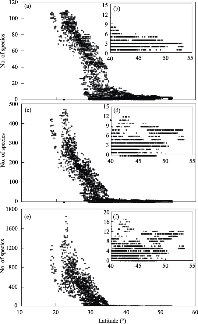
Figure A1 Latitude gradients of (a) families richness, (c) genera richness and (e) species richness of EBWPs in 50 km×50 km grid cells across China. (b), (d) and (f) reflect the detailed information of the latitude gradients of families richness, genera richness and species richness of EBWPs distributed north of 40°N in China. |
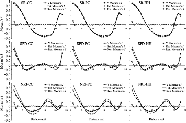
Figure A2 Spatial correlograms for the geographic patterns in species richness (SR), standardized phylogenetic diversity (SPD) and net relatedness index (NRI) of the EBWPs in China, and the estimates and residuals of the combined models. Spatial correlograms are estimated by Moran’s I coefficients. In the figures, solid dots represent Moran’s I for raw data (Y), while crosses and solid dots represent Moran’s I for the estimates and residuals of the explanatory models of current climate (CC), the paleo-climate variation (PC) and that of habitat heterogeneity (HH). |
The authors have declared that no competing interests exist.
| 1 |
|
| 2 |
|
| 3 |
|
| 4 |
|
| 5 |
|
| 6 |
|
| 7 |
|
| 8 |
|
| 9 |
|
| 10 |
|
| 11 |
|
| 12 |
|
| 13 |
|
| 14 |
|
| 15 |
|
| 16 |
|
| 17 |
|
| 18 |
|
| 19 |
|
| 20 |
|
| 21 |
|
| 22 |
|
| 23 |
|
| 24 |
|
| 25 |
|
| 26 |
|
| 27 |
|
| 28 |
|
| 29 |
|
| 30 |
|
| 31 |
|
| 32 |
|
| 33 |
|
| 34 |
|
| 35 |
|
| 36 |
|
| 37 |
|
| 38 |
|
| 39 |
|
| 40 |
|
| 41 |
|
| 42 |
|
| 43 |
|
| 44 |
|
| 45 |
|
| 46 |
|
| 47 |
|
| 48 |
|
| 49 |
|
| 50 |
|
| 51 |
|
| 52 |
|
| 53 |
|
| 54 |
|
| 55 |
|
| 56 |
|
| 57 |
|
| 58 |
|
| 59 |
|
| 60 |
|
| 61 |
|
| 62 |
|
| 63 |
|
| 64 |
|
| 65 |
|
| 66 |
|
| 67 |
|
| 68 |
|
| 69 |
|
| 70 |
|
| 71 |
|
| 72 |
|
| 73 |
|
| 74 |
|
| 75 |
|
| 76 |
|
| 77 |
|
| 78 |
|
| 79 |
|
| 80 |
|
| 81 |
|
| 82 |
|
| 83 |
|
| 84 |
|
| 85 |
|
| 86 |
|
| 87 |
|
| 88 |
|
| 89 |
|
/
| 〈 |
|
〉 |