Orginal Article

The response of spiders to less-focused non-crop habitats in the agricultural landscape along the lower reach of the Yellow River

  • HOU Xiaoyun , 1, 2 ,
  • DING Shengyan , 1, 2, * ,
  • ZHAO Shuang 1, 2 ,
  • LIU Xiaobo 1, 2
Expand
  • 1. Key Laboratory of Geospatial Technology for the Middle and Lower Yellow River Regions, Ministry of Education, Kaifeng 475004, Henan, China
  • 2. College of Environment and Planning, Henan University, Kaifeng 475004, Henan, China

*Corresponding author: Ding Shengyan, Professor, E-mail:

Author: Hou Xiaoyun (1989-), PhD Candidate, specialized in ground arthropods research. E-mail:

Received date: 2018-05-10

  Accepted date: 2019-01-22

  Online published: 2019-07-25

Supported by

National Natural Science Foundation of China, No.41771202, No.41371195

Copyright

Journal of Geographical Sciences, All Rights Reserved

Abstract

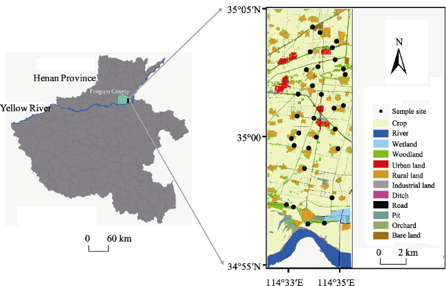
Non-crop habitats have been suggested to impact local biodiversity significantly in agricultural landscapes. However, there have been few studies of the effects of less-focused non-crop habitats (orchard, wetland, pit and ditch) on variation of spider abundance. In this study, spiders in 30 woodlands were captured using pitfall traps in Fengqiu County, China, and the effects of local and landscape variations at different scales (50 m, 100 m, 200 m, 350 m and 500 m) on spider abundance were analysed. The most important variation that influenced spider abundance at the 500 m scale was the less-focused non-crop habitat (LNH) cover, and 10% was an appropriate proportion of LNH cover to sustain high level of spider diversity in the investigated landscape. Non-metric multidimensional scaling analyses revealed that there were significant differences in the spider composition among the high, medium and low LNH coverage. Based on indicator species analysis, different spider species were associated with landscapes with different levels of LNH cover. Lycosidae, which accounted for 48% of the total specimens, preferred woodland habitats neighbouring areas with high LNH cover. Compared with woodland habitats, LNH provided more diverse food sources and habitat to sustain more spider species in the study area. Furthermore, linear elements composed of vegetation, such as pits and ditches, may prevent agricultural intensification by enhancing landscape connectivity and providing habitats for different spiders. Our findings may provide a theoretical basis for biodiversity conservation in agro-ecosystems and top-down control of pests.

Cite this article

HOU Xiaoyun , DING Shengyan , ZHAO Shuang , LIU Xiaobo . The response of spiders to less-focused non-crop habitats in the agricultural landscape along the lower reach of the Yellow River[J]. Journal of Geographical Sciences, 2019 , 29(7) : 1113 -1126 . DOI: 10.1007/s11442-019-1648-4

1 Introduction

An agricultural landscape is a heterogeneous landscape that is composed of non-crop habitats (farmland boundaries, woodland and hedges) and intensified crop fields (Bennett et al., 2006; Kleijn et al., 2009, 2011). Composition heterogeneity is an important element in spatial heterogeneity (Fahrig et al., 2005, 2011). Researches conducted at a large spatial scale often find more obvious ecological processes and interactions than those conducted at a small spatial scale; thus, it was necessary to combine spatial patterns with ecological processes at landscape scale (Steffan et al., 2002).
Biodiversity is essential for ecosystem services (Benton et al., 2003; Carrete et al., 2009; Fu, 1995; MEA, 2005). However, biodiversity shows a downward trend in most regions (Butchart et al., 2010; Jenkins et al., 2003; Kerr et al., 2000; Pereira and Daily, 2006; Pimm and Raven, 2000). An increasing number of researchers have begun to pay attention to biodiversity conservation (Rossi, 2011).
It is widely known that agricultural landscape heterogeneity is closely related to biodiversity (Lazzerini et al., 2007; Schneider et al., 2012), as large numbers of non-agricultural species rely on food and habitats that are provided by agricultural landscape (Liu et al., 2006). Meanwhile, different types of non-crop habitats can increase the heterogeneity of an agricultural landscape, which makes them important for biodiversity conservation (Ekroos et al., 2013; Kleijn and Verbeek, 2000). Therefore, low intensified agricultural landscapes with a high proportion of non-crop habitats are able to sustain greater biodiversity than natural landscapes (Carnus et al., 2006; Ernoult and Alard, 2011; Hartley, 2002; Tscharntke et al., 2005). The impact of landscape heterogeneity on biodiversity has attracted the attention of researchers. Research is performed at the field, landscape, regional, and even national scales (Billeter et al., 2008). Arthropods are an important taxa group of terrestrial ecosystems, and there have been extensively studies conducted on arthropods (Deyn et al., 2003; Robertson et al., 1994; Yin, 2001). Researchers mostly focus on ground arthropods in different types of ecosystems, such as farmland (Zhu et al., 2000; Fournier and Loreau, 2001; Gurr et al., 2003; Li et al., 2004; Zhang et al., 2004; Aviron et al., 2005; Hendrickx et al., 2007; Diekötter et al., 2010; Flohre et al., 2011), grassland (Maharning et al., 2009; Louzada et al., 2010), forest (Bird et al., 2000; Conzúlez and Seastedt, 2001; Lavelle et al., 2006; Huhta, 2007; Heiniger et al., 2014) and so on. Researchers have found that the effects of landscape heterogeneity on ground arthropods vary by scale and that different landscapes have different effects on ground arthropods (Liu et al., 2004; Chang et al., 2012).
Spiders are an important predatory group and biological-control agent of arthropods (Liu et al., 2016). Additionally, spiders are often abundant in temperate agricultural landscapes (Gardiner et al., 2010; Maisonhaute et al., 2010). The study of spiders in agricultural settings is an important link to other research on top-down control of crop herbivores (Karp et al., 2013). To enhance pest control using spiders, a non-crop habitat should be set in agricultural landscapes to facilitate spider migration into crop fields during early spring (Öberg et al., 2008). Although ameliorating non-crop habitats are a way to protect biodiversity of agricultural ecosystems (Carvell et al., 2007; Pryke and Samways, 2009; Li et al., 2013), most non-crop habitats are still forcefully disturbed by human activity, and biodiversity is also confronted with enormous threats (Vackar et al., 2012). In recent years, studies on landscape heterogeneity, biodiversity and ecosystem services have been increased emphasis (Lu et al., 2014; Tang et al., 2014), but the scale effects of non-crop habitats on spiders are rarely studied.
Fengqiu, a county of Henan Province, is a typical agricultural region in the lower reach of the Yellow River, and is dominated by agricultural landscapes. Understanding the relationship between the composition heterogeneity and biodiversity is critical to maintaining ecosystem services and ecosystem stability in this area.
As a research background, the structural composition of woodland sampling sites that surround landscapes across a mosaic agricultural landscape and different types of land uses at five spatial scales, 50, 100, 200, 350 and 500 m radii from the centre of sampling sites, were assessed. Spiders were collected using pitfall traps from each woodland site and were then analyzed in relation to the land use composition. Hence, this study specifically studied whether the abundance and species composition of different spider groups were influenced by variation of LNH among woodland areas and across landscape in heterogeneous agricultural areas. Aims of the study were to investigate: 1) how did the landscape composition impact spider diversity at different scales? 2) in particular, how did LNH cover impact spider diversity? 3) how did different spider species relate to LNH cover?

2 Methodology and data sources

2.1 Study sites

This study was conducted in agricultural landscape of Fengqiu County in northeast Henan Province, China (34°53′-35°14′N, 114°14′-114°46′E). Fengqiu County is a typical agricultural region in the lower reach of the Yellow River and is characterized by a warm temperate continental monsoon climate. The main soil type is yellow fluvo-aquic soil. The average annual rainfall is 615.1 mm, and the average annual temperature is 14 ℃. Landscapes along the Yellow River are mainly alluvial plain characterized by complex habitats and mixed diversity.
Landscape is characterized by a mixture of agricultural fields and more or less non-crop habitats. Agricultural production of annual and perennial cereal crops is the typical land use of this agricultural landscape, with a total area of 81,367 ha, accounting for 66.4% of the total area of the county. The annual crops include corn, wheat, rice and vegetables, while the perennial crops include honeysuckle and raspberry. In this area, farmers sow winter wheat generally at the end of October, and after the harvest of winter wheat, corn is planted continuously. The type of woodland in the study area is an artificial planting of trees with a total area of 8672 ha. Broad-leaved species Populus spp. and Paulownia Sieb. et Zucc. are the most common species, and the dominant herb species are in the Compositae, Gramineae, Leguminosae, Cruciferae and Labiatae families (Lu et al., 2014).

2.2 Study design

A land use map (1:10,000) of Fengqiu was used to identify different habitats across the landscape, and ArcGIS 10.0 was relied upon for further analysis. A total of 30 sampling sites in woodland habitats were selected, and the distances from sites to the road were measured (Figure 1). Combined with field investigation and actual situation of the study area, the landscape was grouped into 12 categories, i.e., crop, woodland, road, urban land, rural land, industrial land, river, wetland, pit, orchard, ditch and bare land.
Figure 1 Distribution map of 30 sampling sites in the study area
Five plastic pitfall traps (7.8 cm in top diameter, 6 cm in bottom diameter, 17.5 cm in depth and 500 ml in volume) were installed at each site. The traps were placed at 10 m intervals and covered with plastic plates to exclude rain water. When the trapping started, the cups were partially filled with 150-200 ml of 20% ethylene glycol and a drop of detergent as a preservative. The traps were collected every 5 days from each site during the periods from 20 April to 6 May and 10 July to 26 July in 2015, and specimens were collected twice from each site during the two periods. All specimens were transferred to vial tubes with 75% alcohol for later identification by sample number. Collected specimens were sorted in the laboratory into the following categories: beetles (Coleoptera), spiders (Araneae), ants (Hymenoptera) and other insects. Spiders were identified at the species level, while the other taxa were identified to the family or order level. Crops, woodlands and LNHs were inventoried at the centre of sites using a 50 m scale and a schematic map of the land use composition. Based on the inventory, the land use map (1:10,000) was used to digitize the types of land use from field-based maps using ArcGIS 10.0 (ESRI, USA).
The maps were used to calculate the land use proportions by estimating the woodland cover and crop cover for each polygon of land use type from satellite images, and then, the total tree cover and crop cover of each site were calculated. Moreover, LNH areas with orchard, wetland, pit and ditch were pooled together. Using the same satellite images, the proportions of different habitats, including the crop cover, woodland cover and LNH cover, of a wider (within 100, 200, 350 and 500 m radii buffer zones around each site) landscape were calculated to determine the effects of different landscape variables at different scales that affected spider abundance (Kiss and Samu, 2000).

2.3 Statistical analysis

Double factor variance analysis was initially used to determine which of the two factors, landscape composition (patch richness) or configuration (patch density), had a greater influence on spider abundance and species richness. Since landscape composition (p < 0.05) was more significant than the configuration (p > 0.05), variables representing the landscape composition at local and landscape scales were chosen as explanatory variables for subsequent analyses (Table 1). The abundance and richness of spiders were treated as response variables in the respective analyses.
Table 1 Explanatory variables at the local (50 m) and landscape (100, 200, 350 and 500 m radii buffers) scales
Variables Spatial scale (m) Range (min-max)% Mean ± SD
Crop cover Local 0-94 27.3±25.3
Woodland cover Local 4-99 63±25.1
Distance from road (m) Local 18.2-1269.5 434.1±397.2
Crop cover Landscape (100 m) 8.1-91.2 44.1±20.3
Woodland cover Landscape (100 m) 3-82 41.4±19.1
LNH cover Landscape (100 m) 0-15.3 3.2±5.4
Crop cover Landscape (200 m) 28-84.5 55.7±14.5
Woodland cover Landscape (200 m) 5.2-56.7 26.2±12.1
LNH cover Landscape (200 m) 0-30 3.4±6.5
Crop cover Landscape (350 m) 35.5-81.5 60.4±11.4
Woodland cover Landscape (350 m) 3-47.7 18.4±9.8
LNH cover Landscape (350 m) 0-24.8 3.6±5.3
Crop cover Landscape (500 m) 38.5-82.6 62.5±10.6
Woodland cover Landscape (500 m) 3.9-42.8 15.5±8.6
LNH cover Landscape (500 m) 0.2-19.8 4.1±6.1
A large variation existed at different scales among most of measured variables (Table 1). For example, the percentage of local crop cover ranged from 0 to 94, while that of woodland cover ranged from 4 to 99. The variance of mean crop cover was the greatest at all the four landscape scales, and the variance of mean LNH cover showed a rising trend when the scales increased.
Before modelling the abundance against landscape variables, the collinearity among measured explanatory variables was tested, and then, all of variables that had no collinearity (Condition Index < 10) were selected for subsequent analyses (Montgomery et al., 2016). Three variables used at the local scale were crop cover, woodland cover and distance from road. At each landscape scale (100, 200, 350 and 500 m), three variables, crop cover, woodland cover and LNH cover, were included for analysis. Owing to the correlation among the landscape variables, only one landscape-scale variable was included in each model, followed by repeated local variable analysis for each of the remaining four landscape variables. Therefore, we used four models: Models 1-4. The best models were those with the lowest Akaike Information Criteria (AIC) values using the stepAIC function within the MASS package (Venables and Ripley, 2002) in the R program (RDCT, 2011). Because of the small sample sizes, AICc was used instead of AIC. The calculated Akaike Weights (Wi) were used to measure the influence of each variable in every model.
We divided the 30 sampling sites into three groups equally based on their LNH cover at the landscape (500 m radius) scale: 1) a high LNH cover (landscape cover > 2.9%); 2) a medium LNH cover; and 3) a low LNH cover (landscape cover < 1.8%) (Figure 2). The logistic fitting method was used to study the effect of LNH cover changes on spider diversity at 500 m scale in MATLAB software. In the following analysis, a non-metric multidimensional scaling analysis (NMDS) based on the lower-triangular dissimilarity matrix in the Vegan package was used to determine differences in the spider composition. Indicator species analysis with the IndVal function was performed to characterize the taxa of spiders in relation to the three groups of LNH cover in the Labdsv package (Dufrêne and Legendre, 1997). Here, indicator value of taxon for a group was calculated based on a combination of its occupancy among sites and relative abundance of the particular group.
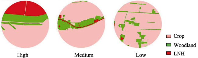
Figure 2 Three LNH cover groups at 500 m scale (each group has only one chosen typical site)

3 Results

3.1 Abundance of spiders

Five hundred sixty-nine spiders (3-56 individuals per site) belonging to 21 taxa and 9 families (Figure 3) were caught. The dominant species were Pardosa astrigena, Hitobia unifascigera, Pirata piratoides and Drassyllus shaanxiensis, accounting for 29.5%, 12.7%, 11.1% and 10.1% of the total individuals, respectively.
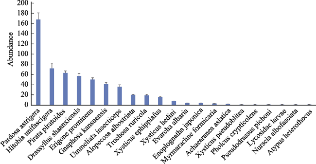
Figure 3 Abundance of spiders

3.2 Response of spider abundance to landscape composition variables at different scales

The statistical models showed a complex interaction between local and landscape variation, which affected abundance of spiders (Table 2). In all models, local variation played an important role in affecting spider abundance, especially crop cover. While crop cover did not have significant effects on the spider abundance at all landscape scales, except at the 100 m scale, neither did woodland cover. LNH cover showed more significant impacts on spiders as the scale increased. For example, the most important variation that influenced spider abundance at the 500 m scale was LNH cover (Wi= 0.36), which replaced local crop cover.
Table 2 Results of the information theoretic model selection and multi-model inference explaining spiders at the local (50 m) and landscape (100, 200, 350 and 500 m) scales
Model Spatial scale Adjusted R2 Loglik df AICc Wi
Model 1 0.177 -5.5798 8 32.2505
Crop cover Local 0.29
Woodland cover Local 0.17
Distance from road (m) Local 0.18
Crop cover Landscape (100 m) 0.21
Woodland cover Landscape (100 m) 0.07
LNH cover Landscape (100 m) 0.06
Model 2 0.052 -7.7082 8 36.5073
Crop cover Local 0.34
Woodland cover Local 0.20
Distance from road (m) Local 0.21
Crop cover Landscape (200 m) 0.09
Woodland cover Landscape (200 m) 0.07
LNH cover Landscape (200 m) 0.08
Model 3 0.148 -6.1067 8 33.3043
Crop cover Local 0.30
Woodland cover Local 0.18
Distance from road (m) Local 0.19
Crop cover Landscape (350 m) 0.06
Woodland cover Landscape (350 m) 0.06
LNH cover Landscape (350 m) 0.21
Model 4 0.170 -5.7152 8 32.5213
Crop cover Local 0.24
Woodland cover Local 0.15
Distance from road (m) Local 0.15
Crop cover Landscape (500 m) 0.05
Woodland cover Landscape (500 m) 0.05
LNH cover Landscape (500 m) 0.36

Notes: Bolded print indicates the most powerful factors in each model.

The following analysis used three categories, High, Medium and Low, to describe LNH cover at 500 m scale. The results indicated that abundance and richness of spiders in woodland were greater in landscapes with a higher LNH cover than those with a lower LNH cover (Figures 4a and 4b).The increasing rate slowed with a LNH cover greater than 10% (Figures 4c and 4d), and 10% might be the best trade-off between set-aside and biodiversity.

3.3 Species composition

We used NMDS to compare differences in spider community composition. The results revealed that each plot had a distinct value from the others based on the lower-triangular dissimilarity matrix calculation (Figure 5). There were significant differences in the species composition of spiders within communities among different scales of LNH cover. Relatively, the spider composition in habitats that had a high LNH cover were more similar to those in habitats that had a medium LNH cover and those in habitats that had a low LNH cover.
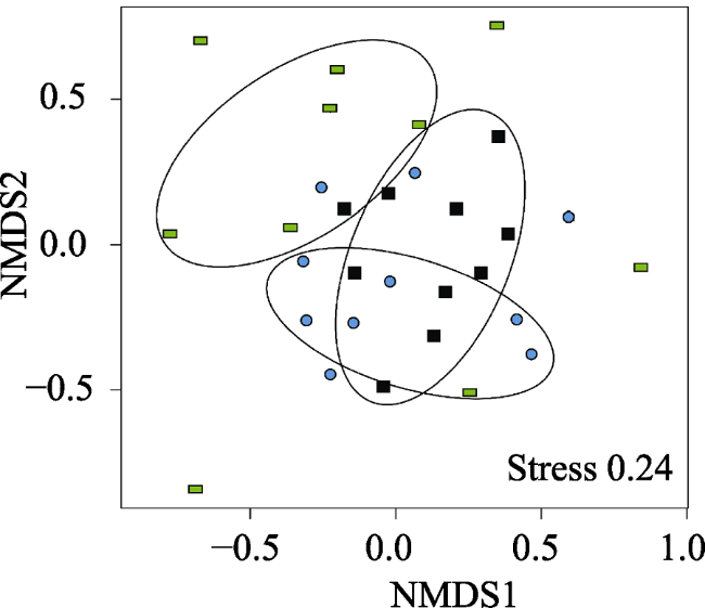
Figure 5 NMDS plot of three categories based on the spider composition at 500 m scale. Black symbols represent plots with a high LNH cover, blue symbols represent plots with a medium LNH cover, and green symbols represent plots with a low LNH cover.
Some 48% of all collected spiders (9 families) were in the Lycosidae family (wolf spiders). Indicator species analysis showed that the majority of spider taxa with a distinct indicator value had higher indicator values in woodland with a high LNH cover (Table 3), especially for spiders in the Lycosidae and Gnaphosidae families. However, a few spider taxa, such as Achaearanea asiatica in the Theridiidae family, Pholcus crypticolens in the Pholcus family, and Lycosidae Larvae in the Lycosidae family, were typical and more frequently appeared in woodland with a medium or low LNH cover (Table 3). According to indicator species analysis, some spider taxa also had a relatively high indicator value (> 0.2), which was associated with a medium or low LNH cover (Table 3). Examples of such taxa were: Pardosa astrigena (Lycosidae), Erigoneprominens (Linyphiidae), Drassyllus shaanxiensis and Hitobia unifascigera (Gnaphosidae). In addition, two spider species were characterized as indicator species (IndVal values between 45% and 70%, Table 3) for the three different levels that were analysed in this study. The indicator species that we identified in this study could be a useful tool for detecting changes of the landscape structure in habitat patches and in the landscape matrix at both levels.
Table 3 Responses of spiders to LNH cover at 500 m scale by indicator species analysis
Taxa Family LNH coverage classes (500 m) and indicator values
Low Medium High
Pardosa astrigena Lycosidae 0.13 0.25 0.49
Pirata piratoides Lycosidae 0.03 0.17 0.29
Trochosa ruricola Lycosidae 0.01 0.08 0.48
Alopecosa albostriata Lycosidae 0 0.02 0.44
Lycosidae Larvae Lycosidae 0.10 0 0
Gnaphosa kansuensis Gnaphosidae 0.10 0.13 0.34
Drassyllus shaanxiensis Gnaphosidae 0.13 0.20 0.40
Hitobia unifascigera Gnaphosidae 0.13 0.21 0.39
Pseudodrassus pichoni Gnaphosidae 0 0 0.10
Erigone prominens Linyphiidae 0.25 0.11 0.30
Ummeliata insecticeps Linyphiidae 0.04 0.14 0.17
Xysticus hedini Thomisidae 0 0.03 0.20
Xysticus ephippiafus Thomisidae 0.11 0.05 0.11
Xysticus pseudoblitea Thomisidae 0 0 0.10
Evarcha albaria Salticidae 0 0.10 0.10
Myrmarachne formicaria Salticidae 0 0.05 0.05
Enoplognatha japonica Theridiidae 0.03 0.03 0.05
Achaearanea asiatica Theridiidae 0 0.10 0
Pholcus crypticolens Pholcus 0 0.10 0
Nurscia albofasciata Titanoecidae 0 0 0.20
Atypus heterothecus Atypidae 0 0 0.10

4 Discussion

4.1 Role of crop cover and LNH cover at different scales

With the change of scales, the responses of spiders also changed. In this study, the most effective landscape variance for spider abundance was crop cover (Local scale) at 100, 200, and 350 m scales (Table 2). Several previous studies agreed with the above findings and suggested that abundance or richness of spiders was related to a local variable (Batáry et al., 2008; Herrmann et al., 2010; Öberg et al., 2008; Schmidt and Tscharntke, 2005; Schmidt et al., 2008). Owing to their natural enemies, spiders often immigrated from the surrounding landscape to arable fields where they controlled pests (Schmidt et al., 2008). Spiders were also influenced by local management practices (ploughing, fertilization, and pest management), agricultural practices (mowing and grazing) and plant and litter cover, which could significantly affect the hunting spider and, to some extent, web-building spider communities (Batáry et al., 2008; Horváth et al., 2015).
The most effective landscape variable affecting the spider abundance shifted to LNH cover at 500 m scale (Wi = 0.36), and spider abundance was positively related to LNH cover (Figure 4c). There existed some researches supporting this result. Schmidt and Tscharntke (2005) found that spider density was positively related to the percentage of non-crop habitats in conventional fields. At the landscape scale, the species richness of spiders was enhanced in non-crop habitats (Schmidt et al., 2008). In smaller spider groups, such as Linyphiid spiders, the abundance was enhanced by high percentages of non-crop habitats in a 1-3 km circumference (Öberg et al., 2008). By contrast, no significant landscape effects were found on abundance and richness of spiders (Batáry et al., 2008). This difference might be due to differences in landscape matrix, the landscape matrix of this study was farmland, while the study of Batáry et al. (2008) was pastures.Therefore, the effect of landscape variance was ignored in this study because local variance produced the most significant effects on spider abundance. The orchard was the landscape matrix used in Herrmann’s study (2010), which led the spider abundance associated with meadow to be affected by plant diversity at the local scale, but not by fragmentation at the landscape scale. The study by Batáry et al. (2008) yielded the same result. In this study, the correlation between spider abundance and LNH cover increased gradually with the increasing scale.
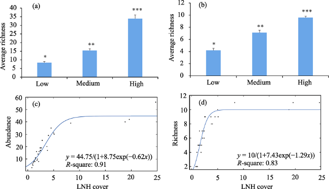
Figure 4 Abundance and richness of spiders in relation to LNH cover (500 m). The three LNH cover classes are based on the combination of orchard, wetland, pit and ditch areas at 500 m scale: 1) high LNH cover (High); 2) medium LNH cover (Medium); and 3) low LNH cover (Low). In the first row (a, b) the symbol (*) among LNH cover classes (High, Medium and Low) indicates significant differences in abundance and richness of spiders. The second row (c, d) shows the logistic trend-line of the abundance (or richness) and LNH cover.

4.2 Spider demand for ecosystem services varies at different scales

Why was the most important variation for spider abundance that of crop cover (50 m) at the 100, 200, 350 m scales, and why did it become a non-crop habitat cover at 500 m scale? What roles did the different habitats play in the effects on spider abundance? It could be speculated that because ecosystem services included supplies, regulations and other services, different ecosystem services might be emphasized for each habitat in agricultural ecosystems, which suggested that the different habitats had their own main ecosystem services (Zhang et al., 2018). In this study, the ecosystem services of the crop habitat for the spider focused on the supply service and the ecosystem services of non-crop habitat, which included woodland and LNH, focused on regulation services (mainly for providing refuge and overwintering sites). The results showed that LNH coverage was low at small scale (100 and 200 m), which provided less regulation services. At this scale, woodland habitats provided regulation services for most spiders, thus, woodland habitats had a high impact on spiderdiversity. The coverage of LNH increased with scale, and the regulation services that could be provided also increased rapidly. LNH provided more regulation services than woodland habitats (the woodland in the study area was artificial woodland and the vegetation cover was rare) at a larger scale. Furthermore, linear elements composed of vegetation-like pits and ditches might prevent agricultural intensification by enhancing landscape connectivity and providing habitats for different spiders. Thus, LNH had a higher impact on spider diversity at larger scales (350 and 500 m) than that at smaller scales (100 and 200 m). Previous studies found that larger spider species were sustained in complex landscapes with a higher availability of refuge and overwintering habitats (Schmidt et al., 2005, 2008).
The results showed that at smaller scales (100, 200 and 350 m), the supply service (provided by local crop cover) was the most important service for spiders, which could allow them to hunt for living prey in crops. Woodland provided the most important regulation service at 100 and 200 m scales. Considerable regulation services were provided to spiders by the landscape LNH cover at 350 and 500 m scales. Especially at 500 m scale, the considerable important variation was LNH cover (Table 2). The results demonstrated that at a greater scale, regulation was more important than supply services for spider abundance and illustrated that the improvement of landscape heterogeneity stimulated the increase of spider abundance in this study area (Figure 4). Therefore, the percentage of non-crop habitat needed to be considered, especially that of LNH cover. However, either mainly in crop habitats (Ricci et al., 2009) or both in crop habitats and non-crop habitats (Rusch et al., 2013), it was found that insect pests respond to the spatial distribution of their host plant resources, so the increased LNH proportion should be limited. Other predatory arthropod families, such as the Carabidae, could be used instead of spiders in future studies.

5 Conclusions

In this study, we studied the multi-scale effects of landscape composition heterogeneity on spider diversity. Our results indicated that the most important variation for spider abundance was that of crop cover (50 m) at 100, 200 and 350 m scales and became LNH cover at 500 m scale. Abundance of spiders was positively related to the LNH cover at 500 m scale, and 10% of LNH cover was appropriate for spider diversity. According to our findings, we believed that the crop habitat could provide a supply service (mainly for food resources) and that woodland and LNH habitats could provide regulation services (mainly for providing refuge and overwintering sites) for spiders. At the large scale, regulation services were more important than supply services for spiders. We should enhance the protection of LNH in the region because regulation services were mainly provided by LNH at the larger scale. This study on spiders contributes to research on top-down pest control, which is more beneficial to agricultural landscape than the use of pesticides. Our research could provide some theoretical guidance for landscape management and biodiversity conservation. Future studies should focus on observing and comparing the response of other predatory arthropod families, such as the Carabidae, to those of spiders in LNH.

The authors have declared that no competing interests exist.

1
Aviron S, Burel F, Baudry J et al., 2005. Carabid assemblages in agricultural landscapes: Impacts of habitat features, landscape context at different spatial scales and farming intensity. Agriculture, Ecosystems and Environment, 108(3): 205-217.

DOI

2
Batáry P, Báldi A, Samu F et al., 2008. Are spiders reacting to local or landscape scale effects in Hungarian pastures?Biological Conservation, 141(8): 2062-2070.

DOI

3
Bennett A F, Radford J Q, Haslem A, 2006. Properties of land mosaics: Implications for nature conservation in agricultural environments. Biological Conservation, 133(2): 250-264.

DOI

4
Benton T G, Vickery J A, Wilson J D, 2003. Farmland biodiversity: Is habitat heterogeneity the key?Trends in Ecology and Evolution, 18(4): 182-188.

DOI

5
Billeter R, Liira J, Bailey D et al., 2008. Indicators for biodiversity in agricultural landscapes: A pan-European study. Journal of Applied Ecology, 45(1): 141-150.

6
Bird S, Coulson R N, Crossley D A J, 2000. Impacts of silvicultural practices on soil and litter arthropod diversity in a Texas pine plantation. Forest Ecology and Management, 131(1): 65-80.

DOI

7
Butchart S H M, Walpole1 M, Collen B et al., 2010. Global biodiversity: Indicators of recent declines. Science, 328(5982): 1164-1168.

DOI

8
Carrete M, Tella J L, Blanco G et al., 2009. Effects of habitat degradation on the abundance, richness and diversity of raptors across Neotropical biomes. Biological Conservation, 142(10): 2002-2011.

DOI

9
Carnus J M, Parrotta J, Brockerhoff E et al., 2006. Planted forests and biodiversity. Journal of Forestry, 104(2): 65-77.

10
Carvell C, Meek W R, Pywell R F et al.F , 2007. Comparing the efficacy of agri-environment schemes to enhance bumble bee abundance and diversity on arable field margins. Journal of Applied Ecology, 44(1): 29-40.

11
Chang H, Zhang X Z, Duan M C et al., 2012. Spatial distribution pattern of carabid assemblage in agricultural landscape of Miyun County, Beijing. Chinese Journal of Applied Ecology, 23(6): 1545-1550.

12
Conzúlez G, Seastedt T R, 2001. Soil fauna and plant litter decomposition in tropical and subalpine forests. Ecology, 82(4): 955-964.

DOI

13
Deyn G B D, Raaijmakers C E, Zommer H R et al., 2003. Soil invertebrate fauna enhances grassland succession and diversity. Nature, 422(6933): 711-713.

DOI

14
Diekötter T, Wamser S, Wolters V et al., 2010. Landscape and management effects on structure and function of soil arthropod communities in winter wheat. Agriculture, Ecosystems and Environment, 137(1-2): 108-112.

15
Dufrêne M, Legendre P, 1997. Species assemblages and indicator species: The need for a flexible asymmetrical approach. Ecological Monograph, 67(3): 345-366.

16
Ekroos J, Kuussaari M, Tiainen J et al., 2013. Correlations in species richness between taxa depend on habitat, scale and landscape context. Ecological Indicators, 34(11): 528-535.

DOI

17
Ernoult A, Alard D, 2011. Species richness of hedgerow habitats in changing agricultural landscapes: Are α and γ diversity shaped by the same factors?Landscape Ecology, 26(5): 683-696.

DOI

18
Fahrig L, Nuttle W K, 2005. Issues and Perspectives in Landscape Ecology. New York, USA: Springer-Verlag.

19
Fahrig L, Baudry J, Brotons L et al., 2011. Functional landscape heterogeneity and animal biodiversity in agricultural landscapes. Ecology Letters, 14(2): 101-112.

DOI

20
Flohre A, Fischer C, Aavik T et al., 2011. Agricultural intensification and biodiversity partitioning in European landscapes comparing plants, carabids, and birds. Ecological Applications, 21(5): 1772-1781.

DOI

21
Fournier E, Loreau M, 2001. Respective roles of recent hedges and forest patch remnants in the maintenance of ground-beetle (Coleoptera: Carabidae) diversity in an agricultural landscape. Landscape Ecology, 16(1): 17-32.

DOI

22
Fu B J, 1995. Landscape diversity analysis and mapping. Acta Ecologica Sinica, 15(4): 345-350.

23
Gardiner M M, Landis D A, Gratton C et al., 2010. Landscape composition influences the activity density of carabidae and arachnida in soybean fields. Biological Control, 55(1): 11-19.

DOI

24
Gurr G M, Wratten S D, Luna J M, 2003. Multi-function agricultural biodiversity: Pest management and other benefits. Basic and Applied Ecology, 4(2): 107-116.

DOI

25
Hartley M J, 2002. Rationale and methods for conserving biodiversity in plantation forests. Forest Ecology and Management, 155(1): 81-95.

DOI

26
Heiniger C, Barot S, Ponge J F et al., 2014. Effect of habitat spatiotemporal structure on collembolan diversity. Pedobiologia, 57(2): 103-117.

DOI

27
Hendrickx F, Maelfait J P, Wingerden W V et al., 2007. How landscape structure, land-use intensity and habitat diversity affect components of total arthropod diversity in agricultural landscapes. Journal of Applied Ecology, 44(2): 340-351.

DOI

28
Herrmann J D, Bailey D, Hofer G et al., 2010. Spiders associated with the meadow and tree canopies of orchards respond differently to habitat fragmentation. Landscape Ecology, 25(7): 1375-1384.

DOI

29
Huhta V, 2007. The role of soil fauna in ecosystems: A historical review. Pedobiologia, 50(6): 489-495.

DOI

30
Horváth R, Magura T, Szinetár C et al., 2015. In stable, unmanaged grasslands local factors are more important than landscape-level factors in shaping spider assemblages. Agriculture, Ecosystems & Environment, 208: 106-113.

31
Jenkins M, Green R E, Madden J, 2003. The challenge of measuring global change in wild nature: Are things getting better or worse?Conservation Biology, 17(1): 20-23.

DOI

32
Karp D S, Mendenhall C D, Sand R F et al., 2013. Forest bolsters bird abundance, pest control and coffee yield. Ecology Letters, 16: 1339-1347.

DOI

33
Kerr J T, Sugar A, Packer L, 2000. Indicator taxa, rapid biodiversity assessment, and nestedness in an endangered ecosystem. Conservation Biology, 14(6): 1726-1734.

DOI

34
Kiss B, Samu F, 2000. Evaluation of population densities of the common wolf spider Pardosa agrestis (Araneae: Lycosidae) in Hungarian alfalfa fields using mark recapture. European Journal of Entomology, 97(2): 191-195.

DOI

35
Kleijn D, Kohler F, Báldi A et al., 2009. On the relationship between farmland biodiversity and land-use intensity in Europe. Proceedings of Biological Sciences, 276(1658): 903-909.

DOI

36
Kleijn D, Rundlöf M, Scheper J et al., 2011. Does conservation on farmland contribute to halting the biodiversity decline?Trends in Ecology and Evolution, 26(9): 474-481.

DOI

37
Kleijn D, Verbeek M, 2000. Factors affecting the species richness of arable field boundary vegetation. Journal of Applied Ecology, 37(2): 256-266.

DOI

38
Lavelle P, Decaëns T, Aubert M et al., 2006. Soil invertebrates and ecosystem services. European Journal of Soil Biology, 42(Suppl.1): S3-S15.

DOI

39
Lazzerini G, Camera A, Benedettelli S et al., 2007. The role of field margins in agro-biodiversity management at the farm level. Italian Journal of Agronomy, 2(2): 127-134.

DOI

40
Li J L, Tang J C, Zhao C Y et al., 2013. Effects of different landscape patch structure on the diversity of arthropod community in tea plantations. Chinese Journal of Applied Ecology, 24(5): 1305-1312.

41
Li L, Tang C, Rengel Z et al., 2004. Calcium, magnesium and microelement uptake as affected by phosphorus sources and interspecific root interactions between wheat and chickpea. Plant and Soil, 261(1/2): 29-37.

DOI

42
Liu X B, 2016. Effects of agricultural landscape structure and habitat characteristics ground-dwelling spiders in typical regions of the lower reaches of the Yellow River [D]. Kaifeng: Henan University.

43
Liu Y, Yu Z, Gu W et al., 2006. Diversity of carabids (Coleoptera, Carabidae) in the desalinized agricultural landscape of Quzhou County, China. Agriculture, Ecosystems and Environment, 113(1-4): 45-50.

DOI

44
Liu Y H, Yu Z R, Liu Y, 2004. Temporal and spatial structure of carabid community in agricultural landscape of Dongbeiwang, Beijing. Chinese Journal of Applied Ecology, 15(1): 85-90.

45
Louzada J, Lima A P, Matavelli R et al., 2010. Community structure of dung beetles in Amazonian savannas: Role of fire disturbance, vegetation and landscape structure. Landscape Ecology, 25(4): 631-641.

DOI

46
Lu X L, Liang G F, Tang Q et al., 2014. Plant species of the non-agricultural habitats in the lower reaches of the Yellow River plain agro-landscape. Acta Ecologica Sinica, 34(4): 789-797.

47
Maharning A R, Mils A A S, Adl S M, 2009. Soil community changes during secondary succession to naturalized grassland. Applied Soil Ecology, 41(2): 137-147.

DOI

48
Maisonhaute J É, Peres-Neto P, Lucas É, 2010. Influence of agronomic practices, local environment and landscape structure on predatory beetle assemblage. Agriculture, Ecosystems and Environment, 139(4): 500-507.

DOI

49
MEA, 2005. Millennium Ecosystem Assessment. Washington: Island Press.

50
Montgomery D C, Peck E A, Vining G G et al., 2016. Introduction to linear regression analysis. 5th ed. Beijing: China Machine Press, 91-268. (in Chinese)

51
Öberg S, Mayr S, Dauber J, 2008. Landscape effects on recolonisation patterns of spiders in arable fields. Agriculture, Ecosystems and Environment, 123(1-3): 211-218.

DOI

52
Pereira H M, Daily G C, 2006. Modeling biodiversity dynamics in countryside landscapes. Ecology, 87(8): 1877-1885.

DOI

53
Pimm S L, Raven P, 2000. Extinction by numbers. Nature, 403(6772): 843-845.

DOI

54
Pryke J S, Samways M J, 2009. Recovery of invertebrate diversity in a rehabilitated city landscape mosaic in the heart of a biodiversity hotspot. Landscape and Urban Planning, 93(1): 54-62.

DOI

55
R Development Core Team (RDCT), 2011. R: A language and environment for statistical computing. R foundation for statistical computing, Vienna, Austria. ISBN 3-900051-07-0, URL .

56
Ricci B, Franck P, Toubon J F et al., 2009. The influence of landscape on insect pest dynamics: A case study in southeastern France. Landscape Ecology, 24(3): 337-349.

DOI

57
Robertson L N, Kettle B A, Simpson G B, 1994. The influence of tillage practices on soil macrofauna in a semi-arid agroecosystem in northeastern Australia. Agriculture, Ecosystems and Environment, 48(2): 149-156.

DOI

58
Rossi J P, 2011. Extrapolation and biodiversity indicators: Handle with caution!Ecological Indicators, 11(5): 1490-1491.

DOI

59
Rusch A, Valantin-Morison M, Sarthou J P et al., 2013. Effect of crop management and landscape context on insect pest populations and crop damage. Agriculture, Ecosystems and Environment, 166(15): 118-125.

DOI

60
Schmidt M H, Roschewitz I C, Tscharntke T, 2005. Differential effects of landscape and management on diversity and density of ground-dwelling farmland spiders. Journal of Applied Ecology, 42(2): 281-287.

DOI

61
Schmidt M H, Thies C, Nentwig W et al., 2008. Contrasting responses of arable spiders to the landscape matrix at different spatial scales. Journal of Biogeography, 35(1): 157-166.

62
Schmidt M H, Tscharntke T, 2005. Landscape context of sheetweb spider (Araneae: Linyphiidae) abundance in cereal fields. Journal of Biogeography, 32(3): 467-473.

DOI

63
Schneider S, Widmer F, Jacot K et al., 2012. Spatial distribution of Metarhizium clade 1 in agricultural landscapes with arable land and different semi-natural habitats. Applied Soil Ecology, 52: 20-28.

DOI

64
Steffan-dewenter I, Münzenberg U, Bürger C et al., 2002. Scale-dependent effects of landscape context on three pollinator guilds. Ecology, 83(5): 1421-1432.

DOI

65
Tang Q, Liang G F, Lu X L et al., 2014. Effects of corridor networks on plant species composition and diversity in an intensive agriculture landscape. Chinese Geographical Science, 24(1): 93-103.

66
Tscharntke T, Klein A M, Kruess A et al., 2005. Landscape perspectives on agricultural intensification and biodiversity ecosystem service management. Ecology Letters, 8(8): 857-874.

DOI

67
Vackar D, Chobot K, Orlitova K, 2012. Spatial relationship between human population density, land use intensity and biodiversity in the Czech Republic. Landscape Ecology, 27(9): 1279-1290.

DOI

68
Venables W N, Ripley B D, 2002. Modern Applied Statistics with S. 4th ed. New York: Springer, .

69
Yin X, 2001. Research of Forest Soil Fauna in Northeast China. Changchun: Northeast Normal University Press.

70
Zhang F, Shen J, Li L et al., 2004. An overview of rhizosphere processes related with plant nutrition in major cropping systems in China. Plant and Soil, 260(1/2): 89-99.

DOI

71
Zhang M Y, Wang K L, Liu H Y et al., 2018. Effect of ecological engineering projects on ecosystem services in a karst region: A case study of northwest Guangxi, China. Journal of Cleaner Production, 183: 831-842.

DOI

72
Zhu Y, Chen H, Fan J et al., 2000. Genetic diversity and disease control in rice. Nature, 406(6797): 718-722.

DOI

Outlines

/