
Journal of Geographical Sciences >
Anthropogenic effect on forest landscape pattern and Cervidae habitats in northeastern China
*Corresponding author: Li Yuehui, E-mail: liyh@iae.ac.cn
Author: Wu Wen, PhD, specialized in landscape ecology. E-mail: wuwen880912@163.com
Received date: 2018-05-10
Accepted date: 2019-01-22
Online published: 2019-07-25
Supported by
National Natural Science Foundation of China, No.41871197, No.41271201
The Doctoral Scientific Research Foundation of Liaoning Province, No.20170520280
The Fundamental Research Funds for the Central Universities of China, No.171104003
Copyright
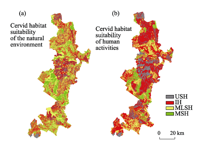
Species abundance and habitat distribution are two important aspects of species conservation studies and both are affected by similar environmental factors. Forest resource inventory data in 2010 were used to evaluate the patterns of habitat for target species of Cervidae in six typical forestry bureaus of the Yichun forest area in the Lesser Xing’an Mountains, northeastern China. A habitat suitability index (HSI) model was used based on elevation, slope, aspect, vegetation and age of tree. These five environmental factors were selected by boosted regression tree (BRT) analysis from 14 environmental variables collected during field surveys. Changes in habitat caused by anthropogenic activities mainly involving settlement and road factors were also considered. The results identified 1780.49 km2 of most-suitable and 1770.70 km2 of unsuitable habitat areas under natural conditions, covering 16.38% and 16.29% of the entire study area, respectively. The area of most-suitable habitat had been reduced by 4.86% when human interference was taken into account, whereas the unsuitable habitat area had increased by 11.3%, indicating that anthropogenic disturbance turned some potential habitats into unsuitable ones. Landscape metrics indicated that average patch area declined while patch density and edge density increased. This suggests that as habitat becomes fragmented and its quality becomes degraded by human activities, cervid populations will be threatened with extirpation. The study helped identify the spatial extent of habitat influenced by anthropogenic interference for the local cervid population. As cervid species clearly avoid human activities, more attention should be paid on considering the way and intensity of human activities for habitat management as fully as possible.
WU Wen , LI Yuehui , HU Yuanman , CHANG Yu , XIONG Zaiping . Anthropogenic effect on forest landscape pattern and Cervidae habitats in northeastern China[J]. Journal of Geographical Sciences, 2019 , 29(7) : 1098 -1112 . DOI: 10.1007/s11442-019-1647-5
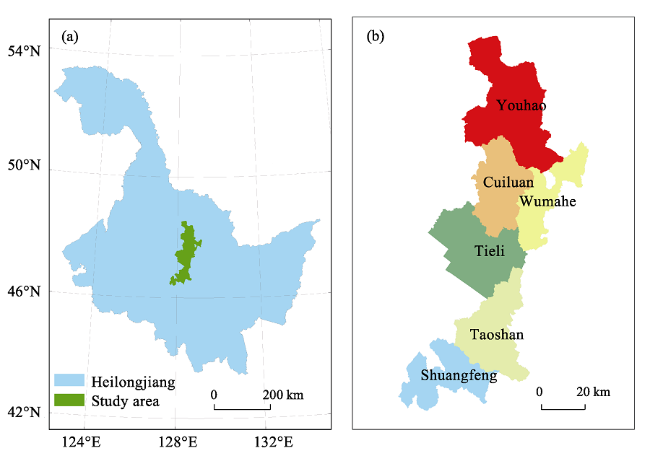
Figure 1 Study area in central Heilongjiang Province, China (a. Study area within Heilongjiang; b. Locations of the six forestry bureaus) |
Table 1 Environmental factors used for boosted regression tree analysis |
| Variables | Data range | Variable type | Measuring method |
|---|---|---|---|
| Elevation | 278.33-648 m | Continuous/Float | GPS |
| Aspect | 0-8 | Classified/Integer | North arrow |
| Slope | 0-18° | Continuous/Integer | Gradiometer |
| Slope position | 0-3 | Classified/Integer | Visual method |
| Food | 0-5 | Classified/Integer | Counting method |
| Age of forest | 0-83 yr | Continuous/Integer | Expert appraisal approach |
| Density of trees | 0-3000/ha | Continuous/Integer | Expert appraisal approach |
| Height of tree | 0-20 m | Continuous/Integer | Altimeter/Expert appraisal approach |
| Shrub coverage | 0-0.8 | Continuous/Float | Counting method |
| Herb coverage | 0-0.9 | Continuous/Float | Counting method |
| Crown density | 0-0.8 | Continuous/Float | Expert appraisal approach |
| Snow depth | 0-40 cm | Continuous/Integer | Ruler of measurement |
| Generation time | 0-600 d | Continuous/Integer | Expert appraisal approach |
| Visibility | 20-200 m | Continuous/Integer | Expert appraisal approach |
Aspect was classified into nine types: 0-flat, 1-north, 2-northeast, 3-east, 4-southeast, 5-south, 6-southwest, 7-west and 8-northwest; Slope position was classified into four types: 0-no slope, 1-upper slope, 2-middle slope and 3-lower slope; Food was classified into five grades: 0, 1, 2, 3 and 4, from small to large abundance |
Table 2 Person correlation coefficients for all pairs of the environmental factors |
| 1 | 2 | 3 | 4 | 5 | 6 | 7 | 8 | 9 | 10 | 11 | 12 | 13 | 14 | 15 | |
|---|---|---|---|---|---|---|---|---|---|---|---|---|---|---|---|
| 1 | 1 | ||||||||||||||
| 2 | -0.231 | 1 | |||||||||||||
| 3 | -0.152 | -0.015 | 1 | ||||||||||||
| 4 | 0.178 | -0.121 | -0.088 | 1 | |||||||||||
| 5 | -0.122 | 0.432 | 0.11 | -0.248 | 1 | ||||||||||
| 6 | 0.002 | 0.147 | 0.016 | 0.164 | 0.141 | 1 | |||||||||
| 7 | -0.098 | 0.664 | 0.005 | 0 | 0.356 | 0.425 | 1 | ||||||||
| 8 | -0.121 | 0.489 | 0.113 | 0.062 | 0.185 | 0.532 | 0.66 | 1 | |||||||
| 9 | -0.055 | 0.153 | 0.068 | 0.165 | 0.199 | 0.484 | 0.402 | 0.467 | 1 | ||||||
| 10 | -0.017 | 0.094 | 0.087 | 0.153 | 0.086 | 0.371 | 0.328 | 0.397 | 0.782 | 1 | |||||
| 11 | -0.116 | 0.182 | 0.006 | 0.033 | 0.312 | 0.282 | 0.267 | 0.275 | 0.35 | 0.163 | 1 | ||||
| 12 | 0.145 | -0.081 | -0.064 | 0.329 | 0.086 | 0.283 | 0.117 | 0.141 | 0.288 | 0.185 | 0.447 | 1 | |||
| 13 | 0.052 | -0.153 | -0.062 | -0.097 | -0.209 | -0.448 | -0.42 | -0.483 | -0.585 | -0.421 | -0.692 | -0.514 | 1 | ||
| 14 | -0.01 | 0.183 | 0.055 | 0.242 | 0.288 | 0.552 | 0.357 | 0.441 | 0.81 | 0.575 | 0.54 | 0.524 | -0.689 | 1 | |
| 15 | -0.09 | 0.288 | 0.111 | 0.21 | 0.281 | 0.435 | 0.429 | 0.463 | 0.632 | 0.437 | 0.445 | 0.502 | -0.621 | 0.704 | 1 |
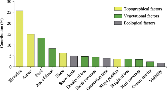
1. Richness of deer; 2. Elevation; 3. Generation time; 4. Food; 5. Snow depth; 6. Aspect; 7. Slope; 8. Slope position; 9. Crown density; 10. Density of trees; 11. Shrub coverage; 12. Herb coverage; 13. Visibility; 14. Height of tree; 15. Age of forest |
Figure 2 Relative influence on the richness of deer for the environmental factors in a boosted regression tree analysis |
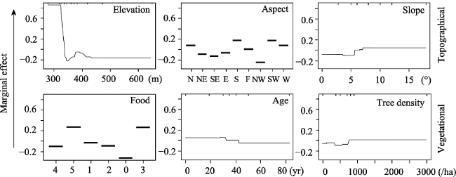
Figure 3 The influence of the main habitat factors on richness of species and dependency points for the first three most important predictor variables of topographical and vegetational factors, respectively, in the boosted regression tree analysis. Food was classified into six grades: 0, 1, 2, 3, 4 and 5, from none to abundant food resources. Age: age of forest |
Table 3 Criteria for suitability assessment of impact factors during the habitat assessment |
| Habitat factors | Most-suitable | Moderately-suitable | Inferior | Unsuitable | |
|---|---|---|---|---|---|
| Geographical | Elevation (m a.s.l.) | 215-300 | 300-500 | 500-700 | 700-1137 |
| Slope (°) | 0-5 | 5-15 | 15-25 | 25-63 | |
| Aspect | S/Flat | SE/SW | E/W/NE | NW/N | |
| Biological | Vegetation | Most-preferred | Moderately-preferred | Preferred | Non-preferred |
| Age (yr) | 30-60 | 60-80 | > 80 | < 30 | |
| Interference | Distance to roads (m) | > 1000 | 500-1000 | 200-500 | 0-200 |
| Distance to settlements (m) | > 1500 | 1000-1500 | 500-1000 | 0-500 | |
Figure 4 Habitat suitability for Cervidae in the study area (a. Cervid habitat suitability based on natural environmental conditions; b. cervid habitat suitability based on human activities. Acronyms: MSH, most-suitable habitat; MLSH, moderately-suitable habitat; IH, inferior habitat; USH, unsuitable habitat |
Table 4 Habitat suitability for Cervidae in the study area |
| Habitat suitability | Natural environment, area (km2) | Human influence, area (km2) | Natural environment, percentage of area (%) | Human influence, percentage of area (%) |
|---|---|---|---|---|
| Most-suitable | 1780.49 | 1252.21 | 16.38 | 11.52 |
| Moderately-suitable | 3216.40 | 2297.89 | 29.59 | 21.14 |
| Inferior | 4102.29 | 4320.78 | 37.74 | 39.75 |
| Unsuitable | 1770.70 | 2999.00 | 16.29 | 27.59 |
Table 5 Spatial index of habitat pattern in the Lesser Xing’an Mountains, northeastern China |
| Habitat | PLAND (%) | AREA_MN (km2) | PD (Patches/km2) | ED (m/km2) | SHAPE_MN | AI | |
|---|---|---|---|---|---|---|---|
| a | MSH | 16.38 | 4.12 | 3.97 | 33.41 | 1.20 | 84.66 |
| MLSH | 29.59 | 3.84 | 7.70 | 67.36 | 1.23 | 82.86 | |
| IH | 37.74 | 4.75 | 7.95 | 61.65 | 1.17 | 87.70 | |
| USH | 16.29 | 6.51 | 2.50 | 25.28 | 1.19 | 88.33 | |
| b | MSH | 11.52 | 2.56 | 4.51 | 22.67 | 1.13 | 85.21 |
| MLSH | 21.14 | 4.58 | 4.61 | 46.82 | 1.20 | 83.33 | |
| IH | 39.75 | 3.75 | 10.60 | 84.21 | 1.14 | 84.06 | |
| USH | 27.59 | 1.30 | 21.19 | 59.03 | 1.09 | 83.91 | |
| Landscape scale | a | 4.52 | 22.13 | 93.85 | 1.20 | 85.87 | |
| b | 2.44 | 40.91 | 106.36 | 1.12 | 83.99 | ||
Acronyms: MSH, most-suitable habitat; MLSH, moderately-suitable habitat; IH, inferior habitat; USH, unsuitable habitat; ED, edge density; a, natural environment, b, anthropogenic influence |
The authors have declared that no competing interests exist.
| 1 |
|
| 2 |
|
| 3 |
|
| 4 |
|
| 5 |
|
| 6 |
|
| 7 |
|
| 8 |
|
| 9 |
|
| 10 |
|
| 11 |
|
| 12 |
|
| 13 |
|
| 14 |
|
| 15 |
|
| 16 |
|
| 17 |
|
| 18 |
|
| 19 |
|
| 20 |
|
| 21 |
|
| 22 |
|
| 23 |
|
| 24 |
|
| 25 |
|
| 26 |
|
| 27 |
|
| 28 |
|
| 29 |
|
| 30 |
|
| 31 |
|
| 32 |
|
| 33 |
|
| 34 |
|
| 35 |
|
| 36 |
|
| 37 |
|
| 38 |
|
| 39 |
|
| 40 |
R Development Core Team (RDCT), 2011. R: A Language and Environment for Statistical Computing. R Foundation for Statistical Computing.
|
| 41 |
|
| 42 |
|
| 43 |
|
| 44 |
|
| 45 |
|
| 46 |
|
| 47 |
|
| 48 |
|
| 49 |
|
| 50 |
|
| 51 |
|
| 52 |
|
| 53 |
|
| 54 |
|
| 55 |
|
| 56 |
|
| 57 |
|
| 58 |
|
| 59 |
|
| 60 |
|
| 61 |
|
| 62 |
|
| 63 |
|
| 64 |
|
/
| 〈 |
|
〉 |