Orginal Article

Potential priority areas and protection network for Yunnan snub-nosed monkey (Rhinopithecus bieti) in Southwest China

  • SU Xukun , 1, 2 ,
  • HAN Wangya 1, 2 ,
  • LIU Guohua , 1, 2, *
Expand
  • 1. State Key Laboratory of Urban and Regional Ecology, Research Center for Eco-Environmental Sciences, CAS, Beijing 100085, China
  • 2. College of Resources and Environment, University of Chinese Academy of Sciences, Beijing 100049, China

*Corresponding author: Liu Guohua, E-mail:

Author: Su Xukun, PhD, specialized in biodiversity conservation and landscape ecology. E-mail:

Received date: 2018-05-10

  Accepted date: 2019-01-22

  Online published: 2019-07-25

Supported by

National Key Research and Development Program of China, No.2016YFC0502102

Copyright

Journal of Geographical Sciences, All Rights Reserved

Abstract

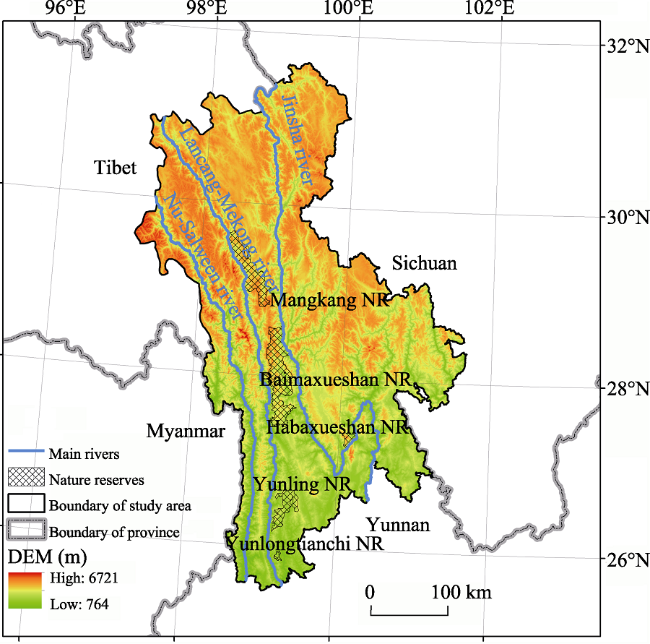
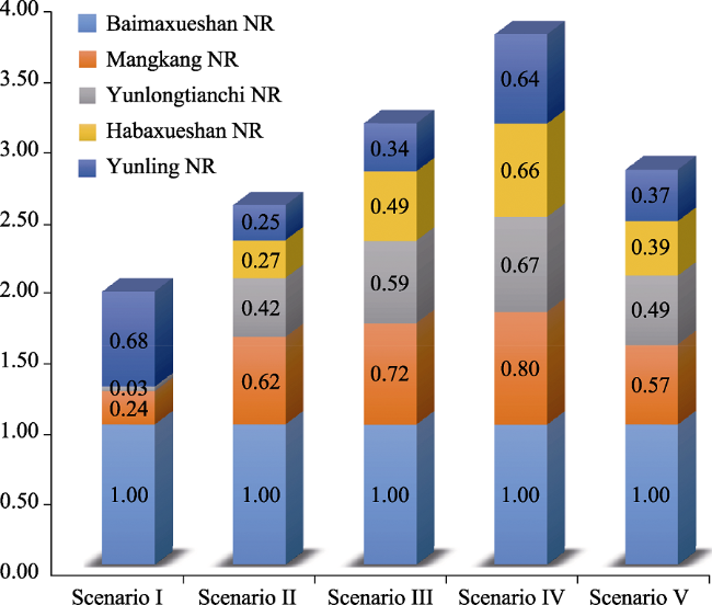
In Southwest China, five Nature Reserves (NRs) (Mangkang, Baimaxueshan, Yunling, Habaxueshan, and Yunlongtianchi) play a key role in protecting the endemic and endangered Yunnan snub-nosed monkey (YSM) (Rhinopithecus bieti). However, increasing human activities threaten its habitats and corridors. We used a GIS-based Niche Model to delineate potential core habitats (PCHs) of the YSMs and a Linkage Mapper corridor simulation tool to restore potential connectivity corridors (PCCs), and defined five scenarios. A normalized importance value index (NIVI) was established to identify the protection priority areas (PPAs) for the YSMs for five scenarios. The results indicated that locations of the habitats and corridors were different in the five scenarios, thereby influencing the distribution of the PPAs and protection network of the YSMs. The NIVI value of Baimaxueshan nature reserve was 1 in the five scenarios, which implied the maximum importance. There were only 7 PCHs and 16 PCCs (with the longest average length of 223.13 km) which were mainly located around 5 NRs in scenario III. The protection network of the YSMs was composed of 16 PCHs, 18 PCCs, and 5 NRs. Under each scenario, most of the PCHs and the PCCs were located in the south of the study area. The five NRs only covered 2 PPAs of the YSMs. We suggest that the southern part of the study area needs to be strictly protected and human activities should be limited. The area of the five NRs should be expanded to maximize protection of the YSMs in the future.

Cite this article

SU Xukun , HAN Wangya , LIU Guohua . Potential priority areas and protection network for Yunnan snub-nosed monkey (Rhinopithecus bieti) in Southwest China[J]. Journal of Geographical Sciences, 2019 , 29(7) : 1211 -1227 . DOI: 10.1007/s11442-019-1654-6

1 Introduction

The Yunnan snub-nosed monkey (YSM) (Rhinopithecus bieti) is an endemic and flagship species in Southwest China, categorized as a Class I Protected Animal under China’s Wildlife Law, and listed as an Endangered Species on the IUCN Red List (Bleisch and Richardson, 2008; Li et al., 2015; Long et al., 1996). Surveys have shown that the YSMs live in 16 isolated groups, with a total of above 3000 individuals in the junction of Yunnan Province, Sichuan Province and Tibet Autonomous Region, from 1800 m to 4700 m elevation (Ren et al., 2016; Wu et al., 2005). The body length of adult YSM ranges from 52 cm to 75 cm, and tail length is between 52 cm and 75 cm. The weight of male YSM (between 15 kg and 17 kg) is heavier than weight of female YSM (between 9 kg and 12 kg) (Ren et al., 2016). Chinese Usnea (Usnea diffracta Vain) and lichens (Bryoria spp.) are main food for the YSMs (Huang et al., 2017; Li et al., 2011). Body hair of the YSM is shiny and gray-black. The YSM can live up to nearly 20 years, generally. The YSMs live and travel in social groups, and the average number of the YSMs in a social group is nearly between 20 and 60. The social groups of the YSMs are generally composed of one-male units and discrete all-male units (Ren et al., 2016).
A considerable amount of evidence has demonstrated the negative effects of human activities on the distribution and abundance of the population, the habitat quality and connectivity of wildlife (Su et al., 2015; Carroll et al., 2012). One of the serious consequences which are attributed to the negative effects of human activities is habitat fragmentation for wildlife. Habitat fragmentation is a spatial process which affect (or potential) core habitats by decreasing their size or increasing their number and/or their isolation of wildlife (Clauzel et al., 2015). Habitat fragmentation of the YSMs is also quite serious due to intensive human activities (such as logging, grazing, mining, agriculture, firewood collecting and other livelihood activities of local people), (Su et al., 2015; Wang et al., 2011; Huang et al., 2017). Because of habitat fragmentation, the YSMs may incur a high energy cost if they travel long distances between core habitat patches (Ren et al., 2009; Ren et al., 2016; Li et al., 2009). The negative effects of habitat fragmentation on wildlife may decrease wildlife diversity directly or indirectly by losing habitat which supports wildlife (Breininger et al., 2012; Li et al., 2015). It may also prevent genetic exchange between populations, making the species more vulnerable to extinction (Grueter et al., 2012; Li and Yang, 2009; Xia et al., 2016; Liu et al., 2009).
Since the 20th century, planned nature reserves (NRs) or protected areas (PAs) which aim to protect wildlife and its habitats have been a cornerstone of conservation methods to minimize the negative effect of human activities and to maximize the positive effects of wildlife protection (Martín-López et al., 2011; Su et al., 2015; Su et al., 2016). Aiming to protect the YSMs and their habitats and reducing habitat fragmentation, the central government of China established five NRs (Mangkang, Baimaxueshan, Yunling, Habaxueshan, and Yunlongtianchi) since the 1980s (Li et al., 2009). However, few researchers have studied the five NRs as a whole to understand the YSMs status in Southwest China, which is one of the most ecologically important areas worldwide. Most of the existing studies only focused on a single nature reserve or a narrow range from Mangkang in Tibet to Yunlongtianchi in the Yunling Mountains, in Yunnan Province which covers an area of approximately 21,000 km2 and extends approximately 350 km from north to south and 60 km from east to west (Li et al., 2015; Wu et al., 2005; Xue et al., 2011; Zhang et al., 2016). As groups of the YSMs are scattered in the Three Parallel Rivers region in a narrow range area with rugged terrain, it is difficult to carry out field surveys (Li et al., 2015; Zhang et al., 2016). Therefore, the distribution area, and movement routes of the YSMs population remain uncertain. Recent news reported that new population of the YSMs was found in the Xiaoping inspection station in the south of Yunlongtianchi NR where the distribution area of the YSMs population is further south by nearly 40 km (http://news.yninfo.com/yn/shxw/201502/t20150213_2321553.html). This evidence indicated that there may be some new populations of the YSMs and potential core habitats which are outside of the narrow range area of the five NRs. Therefore, it is necessary to study the YSMs status and discover new potential core habitats of the YSMs at a large scale.
In addition, corridors among core habitats of wildlife play a key role in maintaining the wildlife population by increasing habitat connectivity, preserving effective population size, promoting gene flow, and facilitating regular migration, dispersal, re-colonization, demographic rescue, and movement in response to climate change (Li et al., 2010; Su et al., 2015; McRae and Kavanagh, 2011). For large mammals such as the YSMs, potential corridors can promote essential ecological processes such as animal movement to increase functional connectivity (Roever et al., 2013; McRae and Kavanagh, 2011). In the study area, there has been little effort towards identifying candidate areas for restoring connectivity corridors across areas that impede wildlife movement (e.g., by removing a fence or building a wildlife-friendly highway underpass). It is detecting restoration opportunities by mapping barriers that strongly reduce movement potential (McRae et al., 2008; McRae et al., 2012). Ideally, not only core habitats of the YSMs should be protected strictly, but also corridors among habitats for improving connectivity should be protected completely. For protecting the YSMs and their habitats completely, it is essential to clarify the distribution of the potential core habitats and connectivity corridors at a large scale, and to identify their priority areas.
We conducted our research in Southwest China to fill the information gaps between single habitat conservation of wildlife and protection network for wildlife which contributes to potential core habitats, connectivity corridors, and the current five NRs. The aims of this study were to: (1) draw locations of potential corridors among the five NRs; (2) clarify distribution of potential core habitats and connectivity corridors of YSMs in different scenarios; (3) identify protection priority areas and protection network.

2 Materials and methods

2.1 Study area

There are five NRs (Mangkang, Baimaxueshan, Yunling, Habaxueshan, and Yunlongtianchi) in the study area. Baimaxueshan NR with an area of 2794 km2, is the largest NR and areas of Mangkang NR, Yunling NR, Habaxueshan NR and Yunlongtianchi NR are 1844 km2, 758 km2, 218 km2, and 65 km2, respectively. We selected 24 counties which surround the five NRs as the study area (Cyril et al., 2010; Cui et al., 2011; Li and Yang, 2009; Long et al., 1996). The study area is located at the junction of three provincial areas of Yunnan, Sichuan, and Tibet in Southwest China bordering Myanmar (Figure 1). With an elevation of 764-6721 m, it covers an area of 143,086 km2 and extends approximately 690 km from north to south and 430 km from east to west. Alpine steppe, alpine meadow and subalpine forest are the dominant land cover types in this area. It is a part of the Three Parallel Rivers Region, where Lancang-Mekong river, Nujiang-Salween river, and Jinsha river run through.
Figure 1 Location of the study area

2.2 Datasets

We selected seven variables including vegetation type, land cover, elevation, slope, aspect, the distance to water, integrating settlement, farmland and road factors for calculating the PCHs of the YSMs (Xue et al., 2011; Zhao et al., 2009; Li et al., 2006). Land cover data (2010) was provided by the “Environmental & Ecological Science Data Center for West China” (http://westdc.westgis.ac.cn). We obtained data on elevation from a Digital Elevation Model (DEM) which was downloaded from the United States Geological Survey (USGS) and derived the slope and aspect from DEM data. The vegetation types of the study area where the YSMs selected as food sources were digitized (Li and Yang, 2009). We derived lakes and rivers to produce water data based on land cover data. We downloaded human activity-related factors which were components of settlement, farmland, mining, and road from Google Maps (Google, Inc.). Using ArcGIS 10.2.2 (ESRI, Redlands, California, USA), we digitized the maps as vector data and formatted all geographical data as raster images in Albers Conical Equal Area projection, with a 90 m/pixel resolution. Finally, we collected 27 points where the YSMs were known to occur from existing research to verify the accuracy of this research (Wu et al., 2005; Shi, 2009; Zhang et al., 2016; Li et al., 2006; Li et al., 2011; Xia et al., 2016).

2.3 Identifying potential core habitats of Yunnan snub-nosed monkey

In order to identify the PCHs of the YSMs, we used the GIS-based niche model (GNM) which incorporated eight environmental and biological factors that were deemed as the most important factors based on the YSMs ecological requirements and natural history (Su et al., 2016; Karanth, 2003; Li et al., 2011; Li et al., 2009; Huang et al., 2017) (Figure 2). Based on previous research and literature, we assigned values from 0 to 100 to seven factors with greater numbers indicating the preference by YSMs(Li et al., 2011; Li et al., 2007; Shi, 2009; Li et al., 2013) (Table 1). For vegetation preferences, several researchers have identified the main plant species in the diets of the YSMs, through analyzing mean relative density percent of plant fragments in feces collected in the field (Li et al., 2011; Li et al., 2009; Li et al., 2007; Zhang et al., 2016). The mean percent of fragments was a proportion of different vegetation types indicating the main food for the YSMs (Li et al., 2011; Li and Yang, 2009). We normalized and assigned these values to different vegetation types. Then we multiplied the seven factors to yield potential core habitats for the YSMs. The resulting maps from the GNM were then reclassified into different kinds of potential habitats for the YSMs, in which 0 (zero) stood for non-habitat, 1-25 for low suitability habitat, 26-50 for moderately suitable habitat, and 51-100 for high suitability habitat (selected as the PCHs).
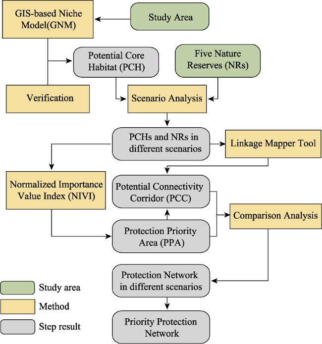
Figure 2 Technical flowchart
Table 1 Weights of each variable
Vegetation types
Name Value Name Value
Tsuga chinensis pritz and Betula alnoides 100 Cotinus nana 50
Tsuga dumosa (D. Don) Eichler 100 Sophora davidii 50
Betula platyphylla Suk 75 Imperata cylindrica 50
Abies delavayi Franch 75 Bothriochloa ischaemum (L.) Keng 50
Betula albo-sinensis Burk. var. septentrionalis Schneid 75 Rhododendron telmateium 50
Platycladus orientalis 75 Arundinella setosa, Arundinella anomala 50
Quercus aquifolioides 75 Rhododendron flavidum Franch 50
bies forrestii 75 Salix cupularis 50
Picea balfouriana 75 Themeda triandra Forsk. Var. Japonica (Willd. )Makino and Miscanthus 50
Neosino calamus affinis 75 Caragana jubata (Pall.) Poir. 50
Larix potaninii var. macrocarpa 75 Rosa sericea Lindl. 50
Sabina tibetica Kom 75 Rhododendron heliolepis Franch. 50
Lithocarpus variolosus (Fr.) Chun 75 Rhododendron delavayi Franch. 50
Castanopsis delavayi Franch 75 Rhododendron fastigiatum Franch. 50
Pinus densata 75 Vaccinium bracteatum Thunb. 50
Quercus pseudosemecarpifolia A. Camus 75 Heteropogon contortus 50
Betula albo-sinensis Burk 75 Malus baccata (L.) Borkh, Prunus padus L. 50
Pinus armandii Franch 75 Rhododendron adenogynum Diels 50
Quercus pannosa Hand.-Mazz. 75 Sabina pingiivar.wilsonii and Sabina squamata 50
Fargesia spathacea Franch 75 Potentilla parvifolia 50
Picea likiangensis 75 Rhododendron nivaleHook. f. 50
Abies squamata Mast 75 Rhododendron racemosum Franch 50
Pinus massoniana Lamb 75 Salix sclerophylla Anderss 50
Quercus guyavaefolia Levl 75 Phyllanthus emblica L. 50
Abies faxoniana Rehd 75 Rhododendron morii Hayata 50
Pobulus davidiana 75 Sibiraea angustata (Rehd.) Hand.-Mazz. 50
Quercus variabilis Bl 75 Kobresia littledalei C. B. Clarke 25
Larix chinensis 75 Carex liparocarpos Gaudin 25
Abies spectabilis (D. Don) Spach 75 Anaphalis flavescens Hand.-Mazz. 25
Castanopsisindica (Roxb.) Miq, Castanopsis clarkei 75 Sanguisorba officinalisL. and Artemisia tanacetifolia Linn. 25
Piceabrachytylavar.omplanata 75 B. sylvaticum (Huds) Beauv 25
Castanopsis concolor Rehd. et Wils. 75 Blysmus sinocompressus Tang et Wang 25
Pinus yunnanensis 75 Cyperaceae 25
Picea asperata Mast. 75 Kobresia humilis and Polygonum macrophyllum D. Don 25
Abies georgei Orr 75 Festuca ovina L. and Deyeuxia arundinacea 25
Pinus palustris Mill. 75 Polygonum macrophyllum D. Don and Polygonum viviparum L 25
Picea purpurea Mast 75 Poa annua L. 25
Quercus monimotricha 50 Non-vegetation 0
Land cover
Name Value Name Value
Forest 100 Wetland 0
Shrub 75 Lake 0
Meadow 25 River 0
Steppe 25 Farmland 0
Vegetation types
Forest wetland 50 Settlement 0
Sparse bushes 50 Road 0
Shrub wetland 0
Aspect
Class Value Class Value
0 0 136°-225° 100
1-45° 25 226°-270° 75
46°-90° 50 271°-315° 50
91°-135° 75
Slope
Class Value Class Value
0 20°-40° 100
0°-90° 25 Above 40° 25
15°-20° 50
Water
Distance Value Distance Value
Water source 0 3.5 km away from water source 50
1 km away from water source 100 More than 3.5 km away from water source 25
Elevation
Class Value Class Value
764-2600 m, 4501-4700 m 25 2801-3600 m 100
2601-2700 m, 4301-4500 m 50 Above 4701 m 0
2701-2800 m, 3601-4300 m 75
Settlement
Class Value Class Value
1 km away from settlement 0 More than 3 km away from settlement 100
3 km away from settlement 50
Road
Distance Value Distance Value
50 m away from road 0 More than 100 m away from road 100
100 m away from road 50

2.4 Scenario analysis

We defined five scenarios to simulate the PCCs among the NRs and PCHs. In scenario I, we selected five NRs as core habitats to identify the PCCs. In scenario II, we selected five NRs and the PCHs with an area of above 100 km2 to generate the PCCs. In scenario III, five NRs and PCHs with an area ranging from 75 km2 to 100 km2 were selected to identify the PCCs since areas in this size range were selected by the YSMs. In scenario IV, five NRs and PCHs with areas between 50 km2 and 75 km2 were selected to identify the PCCs since areas in this size range were selected by the YSMs were used to identify the PCCs. In scenario V, five NRs and all PCHs with area was an area of above 50 km2 were selected to obtain the PCCs.

2.5 Analyzing the potential connectivity corridor

The Linkage Mapper GIS tool was designed to simulate the PCC among habitats (McRae and Kavanagh, 2011; McRae et al., 2012). We used vector data of the PCHs calculated by the GNM method and raster data of movement restricting factors to identify the least-cost linkages among the PCHs. Usually, each cell of a resistance map is given a value reflecting the energetic cost, difficulty, or mortality risk of moving across that cell (Su et al., 2015). Resistance values are typically determined by cell characteristics, such as elevation or human activities (settlement, farmland, and road) and distance to water resources, combined with species-specific landscape resistance models (Beier et al., 2011; Sawyer et al., 2011). Based on existing research, we derived the elevation, slope, and aspect preferred by the YSMs (Xiang et al., 2013; Wu et al., 2005; Li et al., 2013; Li et al., 2009). As the YSMs move away from specific core habitats, cost-weighted distance analyses produce maps of total accumulated movement resistance (McRae et al., 2008). We used the elevation preferred by the YSMs to draw the resistance map. We used buffer analysis to obtain the spatial distribution of the effective range from human activities (settlement, farmland, and road) in the study area. According to the existing research, we selected 1 km, 3.5 km, and 5 km from human activities as buffer distances for all human activities (Xiang et al., 2013). The cell value of the resistance map ranged from 1 (minimum resistance value) to 101 (maximum resistance value).

2.6 Calculating the normalized importance value index (NIVI) of the PCHs

To understand the importance changes of the PCHs and NRs in the different scenarios, we calculated the importance value of each PCH and NR by developing the following formula:
$$\text{IVI=}\frac{\text{A}}{{{\text{T}}_{\text{L}}}}\times {{\text{T}}_{\text{N}}}\ \ \ \ (1)$$
where IVI is the importance value index of the PCHs or NRs in each scenario; A is the area of the PCH or NRs; TL is the total length of all PCCs which connect one PCH or NR; and TN is the total number of the PCCs which connect one PCH or NR. For the IVI comparability among the PCHs or NRs, the IVI of the PCHs and NRs needs to be normalized between zero (no importance) and 1 (the most important) as follows:
$$\text{NIVI=}\frac{\text{IVI-Mi}{{\text{n}}_{\text{IVI}}}}{\text{Ma}{{\text{x}}_{\text{IVI}}}\text{-Mi}{{\text{n}}_{\text{IVI}}}}\ \ \ \ (2)$$
where MinIVI is the minimum importance value of one PCH or NR in each scenario; MaxIVI is the maximum importance value of one PCH or NR; and NIVI is the normalized importance value index of the PCHs or NRs. We used the NIVI to describe the protection importance and priority of the PCHs and NRs in the study area. We selected the PCHs with top 5 NIVI value in each scenario and five NRs as the PPAs to construct protection network of the YSMs.

3 Results

3.1 Distribution of the PCHs in different scenarios and verification

There were 17 points (62.9%) where the YSMs occurred in the five NRs, of which 3 points were in Mangkang NR, 11 points in Baimaxueshan NR, and 3 points were in Yunling NR, respectively. There was no points located in Habaxueshan NR and Yunlongtianchi NR. The 7 points (25.9%) were located in the PCHs, and 2 points in the PCCs; only 1 point was outside of the five NRs, the PCHs, and the PCCs (Figure 3a).
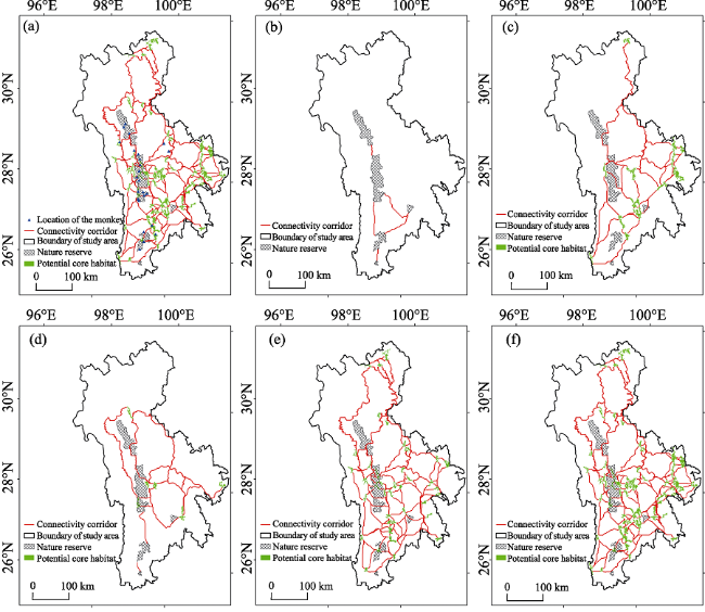
Figure 3 Existing location of the YSMs in the study area (a); location of the PCCs in scenario I (b); distribution of the PCHs and PCCs in scenario II (c); distribution of the PCHs and PCCs in scenario III (d); distribution of the PCHs and PCCs in scenario IV (e); distribution of the PCHs and PCCs in scenario V (f)
Under scenario II, there were 16 PCHs with a total area of 2121 km2 (Table 2). Only one PCH was located at the north of the study area (Figure 3c). Fifteen of 16 PCHs were located in the south of the study area, and only one PCH was in the north. All 7 PCHs with an average area of 90.71 km2 were outside of the five NRs in scenario III (Figure 3d). Under scenario IV, there were 40 PCHs with an average area of 59.90 km2 which was the smallest (Figure 3e). There were 3 PCHs located in the north of study area, 2 PCHs in Baimaxueshan NR, and 1 PCH in Yunling NR. There was a total of 63 PCHs with a total area of 5152 km2, which was the most in scenario V (Figure 3f). There were no PCHs in Mangkang NR, Habaxueshan NR, or Yunlongtianchi NR. Three PCHs were inside Baimaxueshan NR, and 1 PCH inside of Yunling NR.
Table 2 Total number, total area and average area of the PCHs and NRs in different scenarios
Total number Total area (km2) Average area (km2)
Scenario I 5 5679 1135.80
Scenario II 16 2121 132.56
Scenario III 7 635 90.71
Scenario IV 40 2396 59.90
Scenario V 63 5152 81.78

3.2 Distribution of the PCCs in different scenarios

Under scenario I, the total length of all connectivity corridors was 391.68 km (Table 3). There were 5 connectivity corridors with an average length of 78.34 km among 5 NRs. Three connectivity corridors were located among Baimaxueshan NR, Yunling NR, and Habaxueshan NR (Figure 3b). Only 1 connectivity corridor was located between Mangkang NR and Baimaxueshan NR, and between Yunlongtianchi NR and Yunling NR. There was no connectivity corridor between Mangkang NR and Habaxueshan NR, between Habaxueshan NR and Yunlongtianchi NR, between Baimaxueshan NR and Yunlongtianchi NR, directly.
Table 3 Total number, total distance and average length of the PCCs in different scenarios
Total number Total distance (km) Average length (km)
Scenario I 5 391.68 78.34
Scenario II 31 4329.05 139.65
Scenario III 16 3570.07 223.13
Scenario IV 122 12126.41 99.40
Scenario V 182 11842.43 65.07
In scenario II, the distributions of PCHs and PCCs of the YSMs were shown in Figure 3c. There were a total of 16 PCHs with a total area of 2121 km2, and 15 of the 16 PCHs were located in the south of the study area. On the contrary, only one PCH was located in the north of the study area. The total distance, average length and number of the PCCs are listed in Table 2. All PCHs were outside of the five NRs in this scenario. There were one PCC across Mangkang NR, 2 PCCs across Baimaxueshan NR, 1 PCC across Yunlongtianchi NR and Habaxueshan NR, and no PCCs across Yunling NR. There were only 7 PCHs which were located around Mangkang NR, Baimaxueshan NR, and Yunling NR in scenario III (Figure 3d). The total area of the PCHs was 635 km2, and the average area of the PCHs was 90.28 km2. However, only one PCH was inside of Baimaxueshan NR. The total distance and number of the PCCs were 3570.07 km and 16. The average length of the PCCs was 223.13 km, the longest among the 5 scenarios. Only one PCCs was connected between Mangkang NR and Habaxueshan NR, and 3 PCCs were connected across Baimaxueshan NR. There was no PCCs to connect Yunling NR and Yunlongtianchi NR together. Under scenario IV, The total length of all PCCs was 12126.41 km and there were 122 PCCs with an average length of 99.40 km. The total number of the PCHs with a total area of 2568 km2 was 40 (Table 3). However, only 2 PCHs were inside of Baimaxueshan NR, and 1 PCH was inside of Yunling NR (Figure 3e). Three PCHs appeared in north of study area. There were 3 PCCs across Mangkang NR, 12 PCCs across Baimaxueshan NR, 1 PCCs across Habaxueshan NR and Yunlongtianchi NR, and 4 PCCs across Yunling NR. Under scenario V, the average length of the PCCs was the shortest (65.07 km) and the total number of the PCCs was 182. There were 13 PCCs across Baimaxueshan NR, 3 PCCs across Mangkang NR, 3 PCCs across Habaxueshan NR, 5 PCCs across Yunling NR, and 1 PCC across Yunlongtianchi NR, respectively (Figure 3f).

3.3 The NIVI value changes of five NRs in different scenarios

The NIVI value of Baimaxueshan NR was 1 (the maximum value) in each scenario (Figure 4). The NIVI value of Habaxueshan NR was 0 (zero) in scenario I, 0.27 in scenario II, 0.49 in scenario III, 0.66 in scenario IV, and 0.39 in scenario V. The NIVI value of Mangkang NR ranged from 0.24 to 0.8 in five scenarios. The NIVI values of Yunlongtianchi NR were between 0.03 and 0.67 in different scenarios. The NIVI values of Yunling NR were 0.68, 0.25, 0.34, 0.64, and 0.37 in scenario I, II, III, IV, and V, respectively. The total NIVI value of five NRs was the maximum (3.77) in scenario IV, and the minimum (1.95) in scenario I.
Figure 4 The NIVI value changes of the five NRs in each scenario

3.4 Identification of the PPAs and protection network

All five NRs were listed as the PPAs. Locations of the PCHs with the top 5 NIVI values in scenario II, scenario III, scenario IV, and scenario V were shown in Figure 5. A total of 16 PCHs, 5 NRs and 18 PCCs as a protection network of the YSMs were located in south part of study area (Figure 6). There were 5 PCCs across Baimaxueshan NR, 3 PCCs across Yunling NR, 1 PCC across Mangkang NR, Yunlongtianchi NR, and Yunlongtianshi NR, re- spectively.
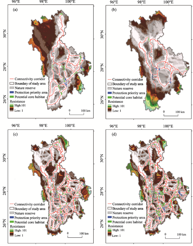
Figure 5 Distribution of the PPAs and the PCCs in scenario II (a), scenario III (b); scenario IV (c), and scenario V (d)
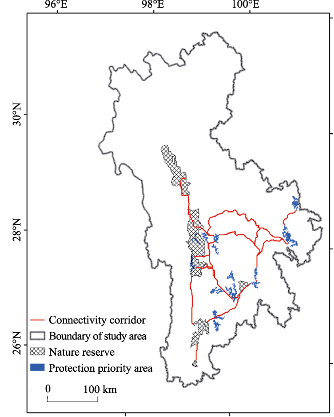
Figure 6 Protection network of the YSMs

4 Discussion

4.1 Potential connectivity corridors among five nature reserves

In recent years, an increasing number of studies have focused on the sustainable development of nature reserves (NRs) with higher biodiversity in Southwest China (Su et al., 2014; Xia et al., 2016; Li et al., 2013; Liu et al., 2014). At the same time, the NRs in Southwest China have been confronted with threats (such as human activities and earthquakes), which can undermine their roles in wildlife conservation (Durán et al., 2013; Su et al., 2015; Li et al., 2015; Cui et al., 2011). It is not an effective approach to study Yunnan snub- nosed monkeys (YSMs) in a single NR or smaller area, especially in habitats isolated by the large rivers (Lancang-Mekong river, Nu-Salween river, and Jinsha river), because the five NRs may be important for genetic exchange among different groups of the YSMs from different NRs (or different habitats). Knowledge of whether the YSMs can swim is important in determining whether they can cross large rivers and other bodies of water that might be found in their potential core habitats (PCHs) and potential connectivity corridors (PCCs).
However, there is no evidence to verify that the YSMs can swim across lakes and large rivers. It is necessary to simulate the PCHs and to draw the PCCs among all PCHs under different scenarios through using models in the study area with considering large rivers and other water bodies as barrier factors to affect habitats of the YSMs. Our results showed that there were 5 PCCs in the five NRs. According to the NIVI value of the five NRs in scenario I, Baimaxueshan NR and Yunling NR were more important for protecting the YSMs and should be protection priority areas and referred to as “stepping stones” connecting with other three NRs. Meanwhile, all PCCs which connected Baimaxueshan NR and Yunling NR should be also listed as priority areas for protection in the future. We suggest that all 5 PCCs should be protected strictly and human activities should be limited in those areas. The five NRs need to be sufficiently large for the long-term conservation of the YSMs in Southwest China, making the landscapes surrounding them equally important to maintain biodiversity and ecosystem services (Zhang et al., 2016; Li et al., 2010; Su et al., 2015).

4.2 Location of potential core habitats and connectivity corridors

In this study, we found that distributions of the PCHs and PCCs were different in the five scenarios. Not only were most of the PCHs and PCCs were in the southern part of the study area in four scenarios (scenario II-V), but also, most of the settlements were located in this area. There are a great deal of conflicts between wildlife protection and human activities in this area (Huang et al., 2017). Therefore, how to balance between wildlife protection and development of society in this part is a key question which needs to be solved as soon as possible (Zhao et al., 2014). The average lengths of the PCCs increased sharply in scenarios II-IV. This indicated that human activities cause the YSMs to migrate longer distance for communicating with other groups of the YSMs in other habitats (scenarios II-IV). Due to the blockage by human activities of the PCCs of the YSMs, the YSMs might stay and maintain their life in the nearby PCHs or NRs. As a consequence, the population of the YSMs might decrease without genetic exchange to other groups of the YSMs in these three scenarios. On the contrary, the average length of the PCCs was minimum (65.07 km) in scenario V. In other words, because more corridors were built to connect the PCHs and the NRs together, the YSMs might cost less energy if they travel shorter distances among core habitat patches and the NRs. We found one PCH with an area above 100 km2 in scenario II, and 2 PCHs (area was between 50 km2 and 75 km2) in scenario IV in the north of the study area. It means that the YSMs might use these three north PCHs for avoiding negative effects of human activities in the future if human activities become stronger in the southern part of the study area. Therefore, we should focus on these three patches which may be “Shelter Islands” for protection of the YSMs in the future. Because of the total number of the PCHs with area between 50 km2 and 75 km2 was the highest at 40 patches, habitat fragmentation is quite severe when placed in the context of protection of the YSMs. Our results showed that most of the PCHs were around Baimaxueshan NR, Habaxueshan NR, and Yunling NR. There was one PCH (with an area above 100 km2) near Baimaxueshan NR, 2 PCHs near Habaxueshan NR, and 2 PCHs near Yunling NR in scenario II. This means that the five NRs will not be big enough to cover all PCHs and PCCs in Southwest China. For maximum protection of the YSMs in this region, we suggest that the NRs should be re-planned in the future with the aims of sustainable development of ecosystem services, regionalizing ecological function zones as an important measure to accelerate regional coordinated development and balancing the development of society and wildlife conservation in Southwest China (Abson et al., 2014).

4.3 Protection priority areas and protection network in the future

In this study, we determined that all PCCs should be completely protected in the five scenarios. When all PCHs were selected as protection targets, the YSMs moved the shortest distance and cost the least energy to communicate with other YSM groups that were located at different areas in Southwest China. However, it is not realistic to strictly protect all PCHs and PCCs in such a large area. Therefore, it is useful to identify the PPAs and restore protection network of the YSMs to enhance the protection efficiency and to balance wildlife protection and its cost in the future (Su et al., 2015; Liu et al., 2014). Protection network of wildlife is crucial for many ecological processes that occur across different spatial and temporal scales, from intra-generational scale foraging to inter-population scale dispersal (Fahrig, 2003; Clauzel et al., 2015). An increasingly popular way of improving and restoring protection network is to model the PCHs and PCCs of wildlife using graph theory which is a set of (potential) core habitats of a given species (called “nodes”) potentially connected by functional relationships (or connectivity corridors) (called “links”) (Clauzel et al., 2015; Galpern et al., 2011). The results showed that a total of 16 PCHs, 18 PCCs and the five NRs were protection network of the YSMs, which should be protected completely. All the 16 PPAs and 18 PCCs are located around or among the five NRs, in other words, the protection network is concentrated in the southeast of the study area. Based on the location of the PPAs, PCCs and the five NRs, it is feasible to build protection network to protect the YSMs in the future. Furthermore, the five NRs are not large enough to protect all habitats (real and potential habitats) and whole population of the YSMs Therefore, it is necessary to build protection network for improving protection efficiency and saving protection cost, and then maintain sustainable development of the YSMs in Southwest China.
In brief, how to balance human activities (society development) and wildlife conservation is still a big challenge in Southwest China, which is one of the 34 biodiversity hotpots in the world (Huang et al., 2017; Fu et al., 2010). Based on the PPAs and protection network, effective conservation of wildlife can be beneficial to mitigate the negative effects of human activities and maintain sustainable development of wildlife in Southwest China.

5 Conclusion

The case study tested whether there were potential core habitats and connectivity corridors of the Yunnan snub-nosed monkey (YSM) besides the existing five nature reserves (NRs) in Southwest China. Scenario analysis showed that the distributions of the PCHs and PCCs of the YSMs are obviously different in different scenarios. A total of 16 PCHs, 18 PCCs, and the five NRs compose the protection network of the YSMs. Baimaxueshan NR is the most important core area to restore protection network of the YSMs. Only 2 PPAs of the YSMs are inside of Baimaxueshan NR. Therefore, the five NRs are not large enough to cover all PPAs of the YSMs. The PCH with an area of 117 km2 is identified in the north of the study area in scenario II. The southern part of the study area, where most of the PCHs and the PCCs in each scenario, and all PPAs are located, needs to be strictly protected and human activities in this area should be reduced in the future.

The authors have declared that no competing interests exist.

1
Abson D J, von Wehrden H, Baumgärtner S et al., 2014. Ecosystem services as a boundary object for sustainability. Ecological Indicators, 103: 29-37.

2
Beier P, Spencer W, Baldwin R et al., 2011. Best science practices for developing regional connectivity maps. Conservation Biology, 25(5): 879-892.

DOI

3
Bleisch W, Richardson M, 2008. Rhinopithecus bieti. The IUCN Red List of Threatened Species 2008.

4
Breininger D R, Mazerolle M J, Bolt M R et al., 2012. Habitat fragmentation effects on annual survival of the federally protected eastern indigo snake. Animal Conservation, 15(4): 361-368.

DOI

5
Carroll C, McRae B H, Brookes A, 2012. Use of linkage mapping and centrality analysis across habitat gradients to conserve connectivity of gray wolf populations in western North America. Conservation Biology, 26: 78-87.

DOI

6
Clauzel C, Deng X Q, Wu G S et al., 2015. Assessing the impact of road developments on connectivity across multiple scales: Application to Yunnan snub-nosed monkey conservation. Biological Conservation, 192: 207-217.

DOI

7
Cui M H, Yang G B, Yang S J, 2011. Protection status and management recommendations on Yunnan snub-nosed monkey in Lanping Yunling Provincial Nature Reserve. Forest Inventory and Planning, 36(4): 43-51. (in Chinese)

8
Cyril C G, Li D Y, Feng S K et al., 2010. Niche partitioning between sympatric rhesus macaques and Yunnan snub-nosed monkeys at Baimaxueshan Nature Reserve, China. Zoological Research, 31(5): 516-522.

9
Durán A P, Rauch J, Gaston K J, 2013. Global spatial coincidence between protected areas and metal mining activities. Biological Conservation, 160: 272-278.

DOI

10
Fahrig L, 2003. Effects of habitat fragmentation on biodiversity. Annual Review of Ecology, Evolution, and Systematics, 34(1): 487-515.

DOI

11
Fu W, Liu S L, Degloria S D et al.2010. Characterizing the “fragmentation-barrier” effect of road networks on landscape connectivity: A case study in Xishuangbanna, Southwest China. Landscape and Urban Planning, 95(3): 122-129.

DOI

12
Galpern P, Manseau M, Fall A, 2011. Patch-based graphs of landscape connectivity: A guide to construction, analysis and application for conservation. Biological Conservation, 144(1): 44-55.

DOI

13
Grueter C C, Li D Y, Ren B P et al., 2012. Food abundance is the main determinant of high-altitude range use in snub-nosed monkeys. International Journal of Zoology, doi: 10.1155/2012/739419.

14
Huang Z P, Scott M B, Li Y P et al., 2017. Black-and-white snub-nosed monkey (Rhinopithecus bieti) feeding behavior in a degraded forest fragment: Clues to a stressed population. Primates, doi: 10.1007/s10329-017-0618-7.

15
Karanth K U, 2003. Tiger ecology and conservation in the Indian subcontinent. Journal of the Bombay Natural History Society, 100: 169-189.

16
Li D Y, Peng Z S, Ren B P et al., 2006. Early autumn habitat selection by the Yunnan snub-nosed monkey (Rhinopithecus biett) in Tacheng, Yunnan. Journal of China West Normal University (Natural Sciences), 27(3): 233-238. (in Chinese)

17
Li D Y, Ren B P, Cyril C G et al., 2009. Seasonal selection of sleeping sites in Yunnan snub-nosed monkeys (Rhinopithecus bieti) at Gehuaqing in Baimaxueshan Nature Reserve. Acta Theriologica Sinica, 29(4): 389-395. (in Chinese)

18
Li D Y, Ren B P, He X M et al., 2011. Diet of Rhinopithecus bieti at Xiangguqing in Baimaxueshan National Nature Reserve. Acta Theriologica Sinica, 31(4): 338-346. (in Chinese)

19
Li D Y, Ren B P, Hu J et al., 2013. Time budgets of Rhinopithecus bieti at Xiangguqing in the Baimaxueshan National Nature Reserve, Northwest Yunnan, China. Acta Theriologica Sinica, 33(3): 223-231. (in Chinese)

20
Li G Q, Yang Y M, Xiao W, 2007. A study on vegetation types of Rhinopithecus bieti habitat. Journal of West China Forestry Science, 36(1): 95-98. (in Chinese)

21
Li H L, Li D H, Li T et al., 2010. Application of least-cost path model to identify a giant panda dispersal corridor network after the Wenchuan earthquake: Case study of Wolong Nature Reserve in China. Ecological Modelling, 221(6): 944-952.

DOI

22
Li L, Xue Y D, Wu G S et al., 2015. Potential habitat corridors and restoration areas for the black-and-white snub-nosed monkey Rhinopithecus bieti in Yunnan, China. Oryx, 49(4): 719-726.

23
Li X Y, Yan S J, 2009. Winter Food Habits of the Yunnan snub-nosed monkey (Rhinopithecus bieti) found at Mt. Longma, Yunnan. Acta Anthropologica Sinica, 28(4): 391-399. (in Chinese)

24
Liu, S L, Deng L, Dong S K et al., 2014. Landscape connectivity dynamics based on network analysis in the Xishuangbanna Nature Reserve, China. Acta Oecologica, 55: 66-77.

25
Liu, S L, Dong Y H, Deng L et al., 2014. Forest fragmentation and landscape connectivity change associated with road network extension and city expansion: A case study in the Lancang River Valley. Ecological Indicators, 36: 160-168.

DOI

26
Liu, Z J, Ren B P, Wu R D, 2009. The effect of landscape features on population genetic structure in Yunnan snub-nosed monkeys (Rhinopithecus bieti) implies an anthropogenic genetic discontinuity. Molecular Ecology, 18(18): 3831-3846.

27
Long Y C, Craig K, Zhong T et al., 1996. Status and conservation strategy of the Yunnan snub-nosed monkey. Chinese Biodiversity, 4(3): 145-152. (in Chinese)

28
Martín-López B, García-Llorente M, Palom I et al., 2011. The conservation against development paradigm in protected areas: Valuation of ecosystem services in the Doñana social-ecological system (southwestern Spain). Ecological Economics, 70(8): 1481-1491.

DOI

29
McRae B H, Dickson B G, Keitt T H et al., 2008. Using circuit theory to model connectivity in ecology, evolution, and conservation. Ecology, 89: 2712-2724.

DOI

30
McRae B H, Hall S A, Beier P et al., 2012. Where to restore ecological connectivity? Detecting barriers and quantifying restoration benefits. Plos One, 7(12): e52604.

DOI

31
McRae B H, Kavanagh D M, 2011. Linkage mapper connectivity analysis software. The Nature Conservancy, Seattle WA. Available at: .

32
Ren B P, Li D Y, Liu Z J et al., 2016. Overview on populations and distribution, home range, diet and conservation status of Yunnan snub-nosed monkeys (Rhinopithecus bieti). Chinese Journal of Zoology, 51(1): 148-150. (in Chinese)

33
Ren B P, Li M, Long Y C et al., 2009. Home range and seasonality of Yunnan snub-nosed monkeys. Integrative Zoology, 4(2): 162-171.

DOI

34
Roever C L, van Aarde R J, Legget K, 2013. Functional connectivity within conservation networks: Delineating corridors for African elephants. Biological Conservation, 157: 128-135.

DOI

35
Sawyer S, Epps C, Brashares J, 2011. Placing linkages among fragmented habitats: Do least-cost path models reflect how animals use landscapes?Journal of Applied Ecology, 48: 668-678.

DOI

36
Shi F Q, 2009. Research on population and distribution of Yunnan snub-nosed monkey in Baimaxueshan Nature Reserve. Inner Mongolia Forestry Investigation and Design, 32(5): 102-105. (in Chinese)

37
Su X K, Dong S K, Liu S L et al., 2014. Effects of land use/land cover change (LUCC) on habitats of Tibetan wild donkey in Aerjin Mountain National Nature Reserve. Chinese Journal of Ecology, 33(1): 141-148. (in Chinese)

38
Su X K, Dong S K, Liu S L et al., 2016. Identifying suitable habitats of three ungulates in Arjinshan National Nature Reserve, China. Journal of Mountain Science, 13(1): 157-168.

DOI

39
Su X K, Liu S L, Dong S K et al., 2015. Effects of potential mining activities on migration corridors of Chiru (Pantholops hodgsonii) in the Altun National Nature Reserve, China. Journal for Nature Conservation, 28: 119-126.

40
Wang Y M, Xue Y D, Xia Y F, 2011. Landscape pattern and its fragmentation evaluation of habitat of Rhinopithecus bieti in Northwest Yunnan. Forest Inventory and Planning, 36(2): 34-37. (in Chinese)

41
Wu R D, Zhou R L, Long Y C et al., 2005. Analysis of suitable habitat for Yunnan Golden Monkey with remote sensing. Remote Sensing Information, (6): 24-28. (in Chinese)

42
Xia F, Zhu P F, Li M et al., 2016. Mating behavior of Yunnan snub-nosed monkeys (Rhinopithecus bieti) at Xiangguqing in Baimaxueshan National Nature Reserve, Yunnan, China. Acta Theriologica Sinica, 36(1): 1-14. (in Chinese)

43
Xiang Z F, Xiao W, Huo S et al., 2013. Ranging pattern and population composition of Rhinopithecus bieti at Xiaochangdu, Tibet: Implications for conservation. Chinese Science Bulletin, 58(16): 1505-1512.

44
XueY D, Li L, Li D Q et al., 2011. Analysis of habitat connectivity of the Yunnan snub-nosed monkeys (Rhinopithecus bieti) using landscape genetics. Acta Ecologica Sinica, 31(20): 5886-5893. (in Chinese)

45
Zhang Y, Li L, Wu G S et al., 2016. Analysis of landscape connectivity of the Yunnan snub-nosed monkeys (Rhinopithecus bieti) based on habitat patches. Acta Ecologica Sinica, 36(1): 51-58. (in Chinese)

46
Zhao H D, Liu S L, Dong S K et al., 2014. Characterizing the importance of habitat patches in maintaining landscape connectivity for Tibetan antelope in the Altun Mountain National Nature Reserve, China. Ecological Research, 29(6): 1065-1075.

DOI

47
Zhao W D, Yang P F, Shen Y S et al., 2009. Study on food item and resource of Rhinopithecus bieti at Tacheng in the Baimaxueshan National Nature Reserve. Chinese Journal of Zoology, 44(3): 49-56. (in Chinese)

Outlines

/