
Journal of Geographical Sciences >
Land use and landscape change driven by gully land consolidation project: A case study of a typical watershed in the Loess Plateau
Author: Li Yurui (1983-), PhD and Associate Professor, specialized in rural geography and land engineering.E-mail: lyr2008@163.com
Received date: 2018-08-20
Accepted date: 2018-10-26
Online published: 2019-04-19
Supported by
National Key Research and Development Program of China, No.2017YFC0504701
National Natural Science Foundation of China, No.41571166, No.41731286
Copyright
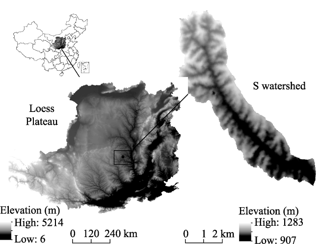
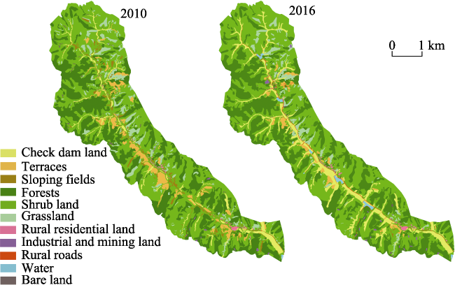
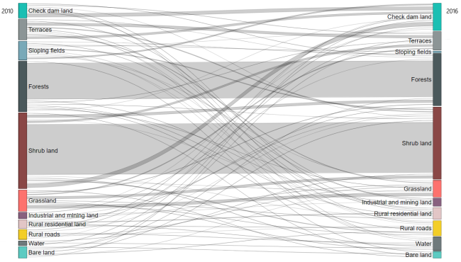
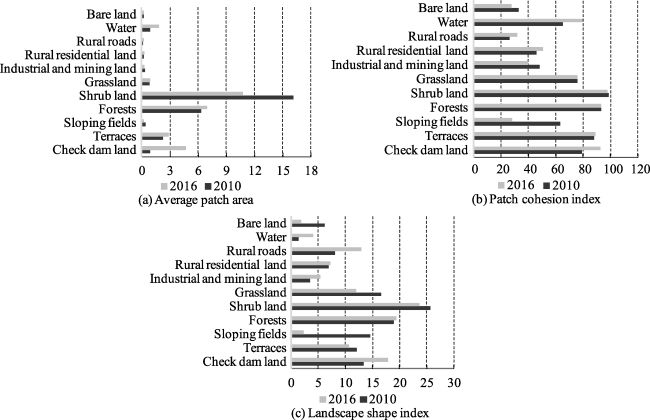
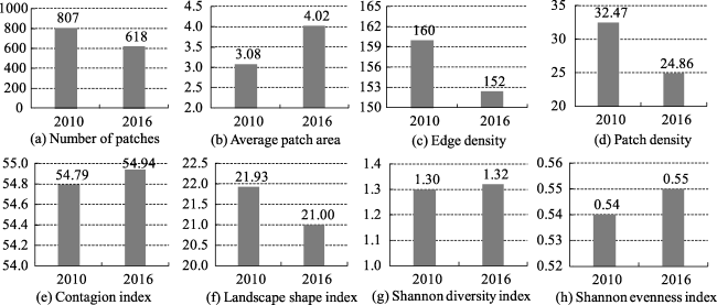
Exploring the impact of land consolidation on the changes of local land use and the landscape patterns is important for optimizing land consolidation models and thus accelerating the sustainable development of local communities. Using a typical small watershed in Yan’an City (Shaanxi, China), the impact of gully land consolidation on land use and landscape pattern change, based on high-resolution remote sensing image data and landscape pattern analysis, was investigated. The results showed that: (1) The terraces, sloping fields, shrub land and grassland at the bottom and both sides of the gully were converted mainly to high quality check dam land. Also, some of the shrub land, due to biological measures, was converted to more ecologically suitable native forest. Thus, the areas of check dam land and forests increased by 159 and 70 ha, while that of shrub land, grassland and sloping fields decreased by 112, 63 and 59 ha, respectively. (2) The average patch area and patch cohesion index for the check dam land increased, which indicated that the production function improved. The landscape shape index and the patch cohesion index for forestland and shrub land were maintained at a high level, and thus the ecological function remained stable. (3) At the watershed level, the degree of fragmentation of the landscape decreased and the landscape became more diversified and balanced; the anti-jamming capability of the landscape and the stability of the ecosystem improved also. Research suggests that implementing gully land consolidation in a rational manner may contribute to improvements in the structure of local land use and the patterns of landscape.
Key words: land consolidation; watershed; land use; landscape; Yan'an City; Loess Plateau
LI Yurui , LI Yi , FAN Pengcan , SUN Jian , LIU Yansui . Land use and landscape change driven by gully land consolidation project: A case study of a typical watershed in the Loess Plateau[J]. Journal of Geographical Sciences, 2019 , 29(5) : 719 -729 . DOI: 10.1007/s11442-019-1623-0
Figure 1 Location and DEM of the study area |
Table 1 Selected landscape indices used in the study |
| Index | Formula | Note | Brief description of index |
|---|---|---|---|
| Average patch area (AREA_MN) | AREA_MN =$\frac{Ai}{Ni}$ | Ni-number of patch type i; Ai-area of patch type i; E-total length of all patch boundaries; A-total landscape area; Pij-total length of edge in landscape between patch types i and k; aij-area of patch i within specified neighborhood of patch j; Ak-total number of cells in the landscape; Pi-proportion of the landscape occupied by patch type i; gik-number of patch i within specified neighborhood of patch type j; m-number of patch types present in the landscape | AREA_MN describes landscape fragmentation. The larger average patch area represents the lower landscape fragmentation. |
| Landscape shape index (LSI) | $LSI=\frac{0.25E}{\sqrt{A}}$ | LSI describes the complexity of landscape shape. The higher the LSI the more complex the shape of the landscape. | |
| Patch cohesion index (COHESION) | $COHESION=\left[ 1-\frac{\sum\limits_{i=1}^{m}{\sum\limits_{j=1}^{n}{Pij}}}{\sum\limits_{i=1}^{m}{\sum\limits_{j=1}^{n}{Pij\cdot \sqrt{aij}}}} \right]\cdot \left[ 1-\frac{1}{\sqrt{A\text{k}}} \right]$ | COHESION describes physical connectivity of the corresponding patch type. The higher the COHESION the stronger the connectivity of the patches. | |
| Number of patches (NP) | NP=Ni | NP describes landscape fragmentation, a landscape with a higher NP would be considered as more fragmented. | |
| Patch density (PD) | PD= | PD describes landscape fragmentation, a landscape with a greater PD would be considered more fragmented. | |
| Edge density (ED) | $ED=\frac{1}{Ai}\sum\limits_{j=1}^{M}{Pij}$ | ED describes landscape fragmentation, a landscape with a greater ED would be considered more fragmented. | |
| Shannon diversity index (SHDI) | $SHDI=-\sum\limits_{i=1}^{m}{\left( Pi In Pi \right)}$ | SHDI describes landscape diversity. A larger SHDI indicates that the landscape has more diverse patch types. | |
| Shannon evenness index (SHEI) | $SHEI=\frac{-\sum\limits_{i=1}^{m}{\left( Pi\cdot In Pi \right)}}{In m}$ | SHEI describes landscape evenness. A smaller SHEI indicates that the landscape is dominated by one or a few dominant patch types. | |
| Contagion index (CONTAG) | $CONTAG=1+\frac{\sum\limits_{i=1}^{m}{\sum\limits_{k=1}^{m}{\left[ \left( Pi \right)\left( \frac{gk}{\sum\limits_{k=1}^{m}{gk}} \right) \right]\cdot \left[ In\left( Pi \right)\left( \frac{gik}{\sum\limits_{k=1}^{m}{gik}} \right) \right]}}}{2In\left( m \right)}$ | CONTAG describes landscape contagion. A larger contagion index indicates that the dominant patch types in the landscape form a good connection. |
Figure 2 Land use change for the S watershed in 2010 and 2016 |
Table 2 Change matrix of each LULC type for the S watershed in 2010 and 2016 and changes in 2016 |
| 2010 (ha) | ||||||||||||||
|---|---|---|---|---|---|---|---|---|---|---|---|---|---|---|
| Type | Check dam land | Terraces | Sloping fields | Forests | Shrub land | Grass- land | Indus- trial and mining land | Rural residential land | Rural roads | Water | Bare land | Sum | Percentage (%) | |
| 2016 | Check dam land | 72.78 | 0.01 | 0.02 | 1.60 | 0.04 | 0.75 | 1.16 | 76.36 | 3.07 | ||||
| Terraces | 45.03 | 54.63 | 3.65 | 15.83 | 10.29 | 0.05 | 0.25 | 2.47 | 3.68 | 135.88 | 5.46 | |||
| Sloping fields | 26.93 | 3.41 | 1.06 | 4.18 | 16.12 | 3.41 | 0.28 | 1.07 | 1.43 | 2.23 | 60.12 | 2.42 | ||
| Forests | 1.15 | 0.14 | 764.01 | 0.83 | 0.04 | 0.57 | 0.01 | 0.02 | 0.05 | 766.82 | 30.83 | |||
| Shrub land | 84.54 | 41.96 | 55.44 | 1063.51 | 3.36 | 2.35 | 1.50 | 11.33 | 6.52 | 0.65 | 1271.16 | 51.11 | ||
| Grass- land | 1.43 | 18.27 | 8.65 | 53.05 | 62.14 | 0.34 | 0.02 | 0.01 | 0.02 | 143.93 | 5.79 | |||
| Indus- trial and mining land | 0.51 | 0.59 | 0.35 | 2.75 | 4.20 | 0.17 | ||||||||
| Rural residential land | 0.25 | 0.20 | 10.48 | 0.20 | 0.02 | 11.15 | 0.45 | |||||||
| Rural roads | 2.98 | 0.01 | 1.63 | 0.26 | 3.69 | 0.77 | 9.34 | 0.38 | ||||||
| Water | 0.15 | 0.01 | 0.80 | 0.96 | 0.04 | |||||||||
| Bare land | 0.18 | 0.40 | 0.11 | 5.42 | 0.92 | 0.03 | 0.15 | 7.21 | 0.29 | |||||
| Sum | 235.42 | 118.83 | 1.06 | 836.57 | 1158.79 | 80.77 | 6.00 | 13.69 | 19.94 | 15.19 | 0.87 | 2487.13 | ||
| Percentage (%) | 9.47 | 4.78 | 0.04 | 33.64 | 46.59 | 3.25 | 0.24 | 0.55 | 0.80 | 0.61 | 0.03 | 100.00 | ||
Figure 3 Flow chart of land use change in the S watershed from 2010 to 2016 |
Figure 4 Changes of landscape structure in the S watershed during 2010 and 2016 |
Figure 5 Changes in the landscape-level metrics from 2010 to 2016 for the S watershed |
The authors have declared that no competing interests exist.
| [1] |
|
| [2] |
|
| [3] |
|
| [4] |
|
| [5] |
|
| [6] |
|
| [7] |
|
| [8] |
|
| [9] |
|
| [10] |
|
| [11] |
|
| [12] |
|
| [13] |
|
| [14] |
|
| [15] |
|
| [16] |
|
| [17] |
|
| [18] |
|
| [19] |
|
| [20] |
|
| [21] |
|
| [22] |
|
| [23] |
|
| [24] |
|
| [25] |
|
| [26] |
|
| [27] |
|
| [28] |
|
| [29] |
|
| [30] |
|
| [31] |
|
| [32] |
|
/
| 〈 |
|
〉 |