
Journal of Geographical Sciences >
Changes in land use/cover mapped over 80 years in the Highlands of Northern Ethiopia
Author: Etefa Guyassa, PhD, specialized in physical geography. E-mail: etefag@gmail.com
Received date: 2017-04-12
Accepted date: 2017-09-13
Online published: 2018-10-25
Copyright
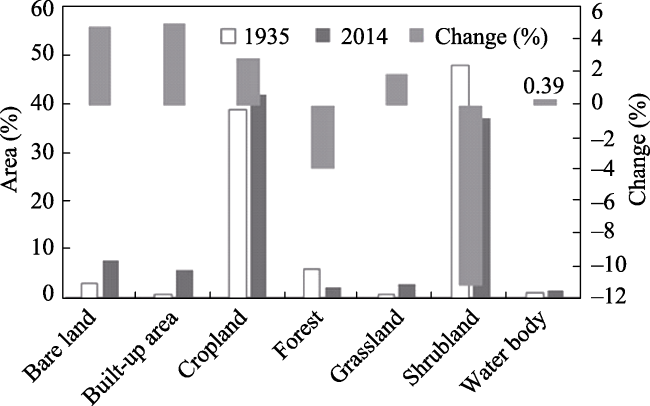
Despite many studies on land degradation in the Highlands of Northern Ethiopia, quantitative information regarding long-term changes in land use/cover (LUC) is rare. Hence, this study aims to investigate the LUC changes in the Geba catchment (5142 km2), Northern Ethiopia, over 80 years (1935-2014). Aerial photographs (APs) of the 1930s and Google Earth (GE) images (2014) were used. The point-count technique was utilized by overlaying a grid on APs and GE images. The occurrence of cropland, forest, grassland, shrubland, bare land, built-up areas and water body was counted to compute their fractions. A multivariate adaptive regression spline was applied to identify the explanatory factors of LUC and to create fractional maps of LUC. The results indicate significant changes of most types, except for forest and cropland. In the 1930s, shrubland (48%) was dominant, followed by cropland (39%). The fraction of cropland in 2014 (42%) remained approximately the same as in the 1930s, while shrubland significantly dropped to 37%. Forests shrank further from a meagre 6.3% in the 1930s to 2.3% in 2014. High overall accuracies (93% and 83%) and strong Kappa coefficients (89% and 72%) for point counts and fractional maps respectively indicate the validity of the techniques used for LUC mapping.
ETEFA Guyassa , Amaury FRANKL , Sil LANCKRIET , BIADGILGN Demissie , GEBREYOHANNES Zenebe , AMANUEL Zenebe , Jean POESEN , Jan NYSSEN . Changes in land use/cover mapped over 80 years in the Highlands of Northern Ethiopia[J]. Journal of Geographical Sciences, 2018 , 28(10) : 1538 -1559 . DOI: 10.1007/s11442-018-1560-3
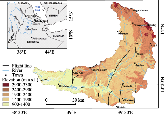
Figure 1 Oro-hydrography of the Geba catchment and flight lines of Italian aerial photographs |
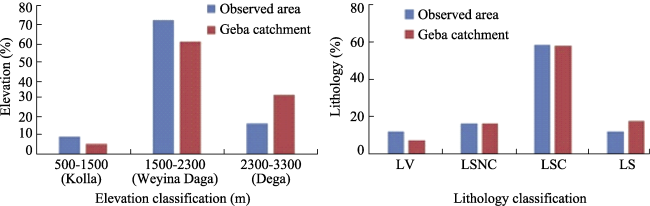
Figure S1 Proportion of elevation (classified based on traditional agro-ecology) and lithology for the observed and predicted map. For explanation on variables see Table 1. |
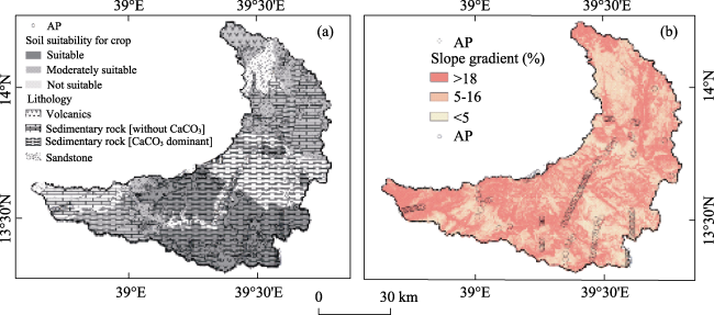
Figure S2 Geba catchment showing: a) lithology (extracted from Tesfamichael et al., 2010; Tesfaye and Gebretsadik, 1982) and soil suitability for cultivation (based on Tielens, 2012); b) slope gradient extracted from DEM - SRTM (USGS, 2014). AP: Location of Italian aerial photo |
Table 1 Variables and their descriptions |
| Factor | Variable | Description | Source/reference |
|---|---|---|---|
| Land use/cover | Bare land | Land with no vegetation cover, rock outcrop, quarry | WBISPP, 2003 |
| Built-up area | Land under settlement, roads | ||
| Cropland | Cultivated land (irrigated and non-irrigated) including open and regularly ploughed with or without shrub or tree line (boundary) and scattered trees, fallow with and without bushes/trees | ||
| Forest | Land covered with dense trees or open; woodland; riparian trees, plantation (large scale and woodlot), church forest | ||
| Grassland | Land covered with grasses used as grazing area | ||
| Shrubland | Land covered with bushes: open, open with trees, dense, dense with trees, exclosures | ||
| Water body | Land covered with water: lake, pond, river including dry river bed | ||
| Topography | Alt (m a.s.l.) | Average elevation at different locations | DEM-SRTM at 30× 30 m resolution |
| Slope (%) | Average slope gradient at different locations. | DEM-SRTM at 30 ×30 m resolution | |
| Soil type | SS | Soils suitable for cultivation, well to perfectly drained, fertile, moderately deep to deep soil. e.g. Vertic Cambisols, Calcaric Vertisols, Vertic Phaeozems | Tielens et al. (2012) |
| SMS | Soils moderately suitable for cultivation, shallow to moderately deep, moderate fertility, moderately drained. e.g. Eutric Regosols, Eutric Cambisols, Calcic Luvisols, Calcaric Cambisols | ||
| SNS | Soils not suitable for cultivation, very shallow, rock outcrop, stony, excessively or poorly drained. e.g. Leptosols, Gleysols | ||
| Lithology | LV | Volcanics (intrusive and extrusive): trap series; Mekelle dolerite. Contain wide range of minerals, which enhance growth of tree and crop | Tesfamichael et al. (2010); Tesfaye and Gebretsadik (1982) |
| LSC | Sedimentary rock dominated by calcium carbonate: metalimestone; Antalo limestone; Agula shale. The land has a dry aspect because of karst and high infiltration. | ||
| LSNC | Sedimentary rocks (non-carbonate): slates, metavolcanics; Edaga Arbi glacials; alluvium. Fine-texture, results in slow infiltration and relatively fertile soils | ||
| LSS | Sandstones: metaconglomerate; major intrusive (these are granites); Enticho sandstone; Amba Aradom sandstone; Adigrat sandstone. These rocks have coarse texture, silica dominated. Sandy weathering materials where water will easily infiltrate; the domination of Si further makes that few minerals are available for vegetation growth | ||
| Socio-economy | Pd (#/km2) | Population density in 2010 | CIESIN, 2016 |
| DT (km) | Distance to town in the 1930s (DT30 and distance to town in 2014 (DT14) | ||
| DR14 (km) | Distance to road in 2014 |
Table 2 Commission-omission error matrix of LUC point count and mapping |
| Ground control / Google Earth | |||||||
|---|---|---|---|---|---|---|---|
| Cropland | Shrubland | Forest | Other cover | Sum | Commission error | ||
| LUC count on screen | Cropland | 132 | 1 | 0 | 2 | 135 | 0.02 |
| Shrubland | 6 | 88 | 3 | 2 | 99 | 0.13 | |
| Forest | 0 | 0 | 6 | 0 | 6 | 0.00 | |
| Other | 3 | 2 | 0 | 30 | 35 | 0.10 | |
| Sum | 141 | 91 | 9 | 34 | 275 | ||
| Omission error | 0.06 | 0.03 | 0.33 | 0.12 | |||
| Overall accuracy | 0.93 | ||||||
| Kappa coefficient | 0.89 | ||||||
| LUC map | Cropland | 106 | 10 | 1 | 6 | 123 | 0.16 |
| Shrubland | 12 | 68 | 1 | 1 | 82 | 0.21 | |
| Forest | 1 | 1 | 3 | 0 | 5 | 0.67 | |
| Other | 4 | 2 | 0 | 17 | 23 | 0.35 | |
| Sum | 123 | 81 | 5 | 24 | 233 | ||
| Omission error | 0.14 | 0.16 | 0.40 | 0.29 | |||
| Overall accuracy | 0.83 | ||||||
| Kappa coefficient | 0.72 | ||||||
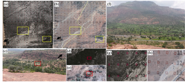
Figure 2 An example of a point grid superimposed on: a) aerial photograph of January 3, 1936 with coordinate of center of vertical photo 13.561547°N and 39.024014°E (i.e. south of Abiy Adi); b) Google Earth image of January 4, 2014. Significant conversion of LUC occurred at this location as shown by: c) terrestrial photo around grid point N16 where land cover changed from dense forest in 1936 (d) to open forest in 2014 (e), and f) terrestrial photo around grid point F12 where land cover changed from open forest in 1936 (g) to cropland with trees in 2014 (h) |
Figure 3 Areal percentage of different land use/cover types in the 1930s and 2014 (n = 34192) |
Table 3 Land use/cover transformation matrix from the 1930s to 2014 in Geba catchment |
| 1935/ 2014 | Cropland | Shrub land | Forest | Grazing land | Built-up | Bare land | Water body | Total |
|---|---|---|---|---|---|---|---|---|
| Cropland | 9047 | 2193 | 116 | 434 | 920 | 714 | 168 | 13592 |
| Shrub land | 4195 | 9151 | 351 | 460 | 680 | 1701 | 289 | 16827 |
| Forest | 514 | 861 | 84 | 36 | 123 | 80 | 17 | 1715 |
| Grazingland | 125 | 95 | 12 | 18 | 85 | 21 | 6 | 362 |
| Bare land | 265 | 410 | 12 | 23 | 60 | 226 | 23 | 1019 |
| Built-up | 79 | 29 | 4 | 7 | 117 | 10 | 1 | 247 |
| Water body | 67 | 177 | 5 | 7 | 40 | 75 | 59 | 430 |
| Total | 14292 | 12916 | 584 | 985 | 2025 | 2827 | 563 | 34192 |
Table 4 Relative importance of variables in the model using three criteria number of subset (the number of model subset that includes the variables), RSS (the scaled summed decrease of residual sum of squares overall subset) and Generalized Cross Validation (GCV). For the explanation on the variables see Table 1 |
| 1930s | 2014 | |||||||
|---|---|---|---|---|---|---|---|---|
| Predictor | Number of subset | GCV | RSS | Predictor | Number of subset | GCV | RSS | |
| Cropland | SS | 7 | 100 | 100 | SS | 8 | 100 | 100 |
| DT30s | 6 | 75 | 77 | Pd | 7 | 66 | 69 | |
| Slope | 6 | 75 | 77 | Slope | 6 | 55 | 59 | |
| Alt | 2 | 17 | 26 | Alt | 5 | 30 | 39 | |
| SMS | 1 | 12 | 18 | SMS | 2 | 4 | 18 | |
| GCV R2 = 0.52 R2 = 0.64 | GCV R2 = 0.63 R2 = 0.73 | |||||||
| Shrubland | Alt | 3 | 100 | 100 | SS | 5 | 100 | 100 |
| Slope | 2 | 54 | 58 | Slope | 4 | 51 | 55 | |
| SNS | 1 | 28 | 33 | Alt | 3 | 32 | 38 | |
| SMS | 1 | 13 | 18 | |||||
| GCV R2 = 0.38 R2 = 0.44 | GCV R2 = 0.58 R2 = 0.64 | |||||||
| Forest | Slope | 6 | 100 | 100 | Alt | 6 | 100 | 100 |
| Alt | 6 | 100 | 100 | LSC | 6 | 100 | 100 | |
| SNS | 6 | 100 | 100 | Pd | 6 | 100 | 100 | |
| LSC | 4 | 36 | 49 | SS | 6 | 96 | 97 | |
| LSNC | 2 | 25 | 34 | |||||
| GCV R2 = 0.40 R2 = 0.52 | GCV R2 = 0.31 R2 = 0.47 | |||||||
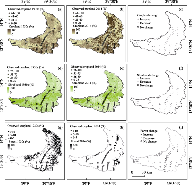
Figure 4 The spatial distribution and change of three dominant land use/cover of the study area: Cropland (a-c), shrubland (d-f) and forest (g-i). A positive (+) and negative (-) sign in these figures indicates the spatial expansion and shrinkage of LUC types, respectively. Graduated classifications illustrate the percent occurrence of land use type in the 1930s and 2014 that also reveal the degree of spatial changes within each location. Sd, Sf1, Sf2, Sh and Ss are supplementary data at Dergajen, Dessa forest 1, Dessa forest 2, Hadinet and Sinkata respectively. |
Table S1 Keys used for the classification of LUC during the point counting on AP and GE |
| Major class | Details class | Description | |
|---|---|---|---|
| X | Impossible to interpret (clouds, damage to photo, poor scan quality) |  | |
| U | Unsure, unknown land cover class | ||
| Bare land | B | Bare (bare soil, rock outcrop), mining area | |
| Cropland | C0 | Cropland fallow (scattered small shrubs) |  |
| C1 | Cropland (open, regularly ploughed) | ||
| C2 | Cropland with shrub or tree line (on lynchet or boundary) | ||
| C3 | Cropland with scattered trees | ||
| Forest | F0 | Forest - open; woodland |  |
| F1 | Forest - dense | ||
Grazing land | G | Grassland |  |
Built-up | H | Habitat (homestead, houses), road | 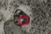 |
| Shrubland | S0 | Shrubland - open | 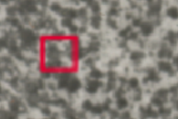 |
| S1 | Shrubland - open - with trees | ||
| S2 S3 | Shrubland - dense Shrubland - dense - with trees | ||
| Water body | W | Water (lake, river, dry river bed, reservoir) | 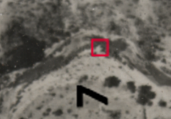 |
Table S2 Frequency and percentage of scene at which land use/cover types have shown different changes between the 1930s and 2014; Chi-square test result. n = 139 |
| Land use/cover | Increased | Decreased | No change | Sig. | |||
|---|---|---|---|---|---|---|---|
| Frequency | Percent | Frequency | Percent | Frequency | Percent | ||
| Bare land | 101 | 73 | 23 | 17 | 15 | 11 | <0.001 |
| Built-up area | 113 | 81 | 17 | 12 | 9 | 6 | <0.001 |
| Cropland | 85 | 61 | 52 | 37 | 2 | 1 | <0.001 |
| Forest | 33 | 24 | 53 | 38 | 53 | 38 | 0.088 |
| Grassland | 96 | 69 | 14 | 10 | 29 | 21 | <0.001 |
| Shrubland | 29 | 21 | 105 | 76 | 5 | 4 | <0.001 |
| Water body | 73 | 53 | 28 | 20 | 38 | 27 | <0.001 |
Table S3 Equations of three major land use/cover (cropland, shrubland and forest) in the 1930s and 2014 which were developed by Multivariate Adaptive Regression Spline model. C1930s = cropland in the 1930s, C2014 = cropland in 2014, S1930s = shrubland in the 1930s, S2014 = shrubland in 2014, F1930s = forest in the 1930s and F2014 = forest in 2014. h=hinge function with zero and a constant (knot) of a factor. For the explanation see Table 1. |
| Land use/cover | 1930s | 2014 |
|---|---|---|
| Cropland | C1930s = 0.2232 - 0.01063 * h (0, DT30s - 6) + 0.02519 * h (0, 17.4 - slope) - 0.1589 * h (0, DT30s - 8) * SS + 0.09218 * h (0, 6 - DT30s) * SMS + 0.04719 * h (0, 7 - slope) * SS - 0.00141 * h (0, 2037 - alt) * SS + 0.1724 * h (0, DT30s - 6) * SS | C2014 = 0.1196 + 0.2177 * SS + 0.0008321 * h(0, alt - 1859) + 0.02293 * h(0, 16 - slope) - 0.000121 * Pd * SS - 0.0000118 * Pd * h (0, 16 - slope) + 0.0005874 * h (0, 1859 - alt) * SMS - 0.0000299 * h (0, alt - 1859) * h (0, slope - 7) - 0.0001047 * h (0, alt - 2150) * h (0, 16 - slope) |
| GCV 0.041 RSS 4.281 GCV R2 0.53 R2 0.64 | GCV 0.028 RSS 2.78 GRSq 0.63 R2 0.73 | |
| Shrubland | S1930s = 0.6112 + 0.1556 * SNS - 0.000357 * h (0, alt - 1778) - 0.01745 * h (0, 15.4 - slope) | S2014 = 0.6841 - 0.2899 * SS - 0.1131 * SMS - 0.0003771 * h (0, 1778 - alt) - 0.0002857 * h (0, alt1 - 1859) - 0.02089 * h (0, 14 - slope) |
| GCV 0.044 RSS 5.441 GCV R2 0.38 R2 0.44 | GCV 0.027 RSS 3.16 GCV R2 0.58 R2 0.64 | |
| Forest | F1930s = 0.06381 + 0.08914 * LSNC - 0.0001301 * h (0, 2361 - alt) + 0.0001466 * h (0, slope - 6) * h (0, alt - 1980) + 0.0001778 * h (0, slope - 6) * h (0, - 2053) + 0.0001651 * slope * max (0, alt - 2361) * LSC + 0.000121 * h (0, slope - 6) * h (0, alt - 1980) * SNS | F2014 = 0.006373 - 0.1273 * SS + 0.0002263 * h (0, alt - 1830) + 0.0003854 * h (0, alt - 2396)* SNS *LSC + 0.02682 * h (0, alt - 2396) * LSC + 0.000000614 * h (0, 2396 - alt) * h (0, Pd - 81) |
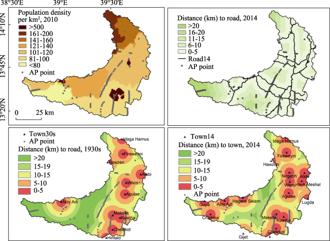
Figure S3 Maps of socio-economic variables |
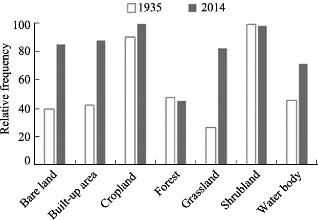
Figure S4 Frequency of occurrence (absence or presence) of different land use/cover types in the 1930s and 2014 scenes, n = 139 |
The authors have declared that no competing interests exist.
| [1] |
|
| [2] |
|
| [3] |
|
| [4] |
|
| [5] |
|
| [6] |
|
| [7] |
|
| [8] |
|
| [9] |
|
| [10] |
|
| [11] |
CIESIN (Center for International Earth Science Information Network)- Columbia University,2016. Gridded Population of the World, Version 4 (GPWv4): Population Density Adjusted to Match 2015 Revision UN WPP Country Totals.Palisades, NY: NASA Socioeconomic Data and Applications Center (SEDAC). Accessed 20 March 2016.
|
| [12] |
|
| [13] |
CSA, 2008. Summary and Statistics Report of the 2007 Population and Housing Census. Federal Democratic Republic of Ethiopia Population Census Commission. December 2008, Addis Ababa, Ethiopia, pp113.
|
| [14] |
|
| [15] |
|
| [16] |
|
| [17] |
|
| [18] |
|
| [19] |
FAO, 2010. Global Forest Resources Assessment: Main report. Foresty paper 163, FAO. Rome, Italy.
|
| [20] |
FAO, 2011. Food and Agriculture Organization Ethiopia Country Programming Framework: 2012-2015. Office of the FAO Representative in Ethiopia to AU and ECA, Addis Ababa.
|
| [21] |
|
| [22] |
|
| [23] |
|
| [24] |
Frankl, A,
|
| [25] |
|
| [26] |
|
| [27] |
|
| [28] |
|
| [29] |
|
| [30] |
|
| [31] |
|
| [32] |
|
| [33] |
|
| [34] |
|
| [35] |
|
| [36] |
HTS, 1976. Tigrai Rural Development Study, Annex 1. Land and Vegetation Resources. Hunting Technical Services Ltd: Hemel Hempstead.
|
| [37] |
|
| [38] |
|
| [39] |
|
| [40] |
IGM. Instituto Geografico Militare, Ente Cartografico dello Stato, 2012. www.igmi.org. Accessed 10 January 2016.
|
| [41] |
|
| [42] |
|
| [43] |
|
| [44] |
|
| [45] |
|
| [46] |
|
| [47] |
|
| [48] |
|
| [49] |
|
| [50] |
|
| [51] |
|
| [52] |
MEA, 2005. Ecosystem and Human Well-being:Synthesis. Millennium Ecosystem Assessment, 2005. Washington DC: : Island Press.
|
| [53] |
|
| [54] |
|
| [55] |
|
| [56] |
|
| [57] |
|
| [58] |
|
| [59] |
|
| [60] |
|
| [61] |
|
| [62] |
|
| [63] |
|
| [64] |
|
| [65] |
|
| [66] |
|
| [67] |
|
| [68] |
|
| [69] |
|
| [70] |
|
| [71] |
|
| [72] |
|
| [73] |
|
| [74] |
|
| [75] |
|
| [76] |
|
| [77] |
|
| [78] |
|
| [79] |
|
| [80] |
|
| [81] |
|
| [82] |
|
| [83] |
USGS, 2016. Shuttle Radar Topography Mission (SRTM)(1-arc second) documentation. 2016.
|
| [84] |
|
| [85] |
|
| [86] |
|
| [87] |
|
| [88] |
|
| [89] |
WBISPP (Woody Biomass Inventory and Strategic Planning Project), 2003. Tigray Regional State: A strategic plan for the sustainable development, conservation, and management of the woody biomass resources. Final Report, Mekelle, Ethiopia.
|
| [90] |
|
| [91] |
|
/
| 〈 |
|
〉 |