
Journal of Geographical Sciences >
Visualization and quantification of significant anthropogenic drivers influencing rangeland degradation trends using Landsat imagery and GIS spatial dependence models: A case study in Northeast Iran
Author: Omid Abdi (1981-), PhD Candidate, specialized in GIS, remote sensing and natural resources. E-mail: omid.abdi@mailbox.tu-dresden.de; oidabdi@gmail.com
Received date: 2016-07-15
Accepted date: 2017-03-27
Online published: 2018-12-20
Copyright
Developing countries must consider the influence of anthropogenic dynamics on changes in rangeland habitats. This study explores happened degradation in 178 rangeland management plans for Northeast Iran in three main steps: (1) conducting a trend analysis of rangeland degradation and anthropogenic dynamics in 1986-2000 and 2000-2015, (2) visualizing the effects of anthropogenic drivers on rangeland degradation using bivariate local spatial autocorrelation (BiLISA), and (3) quantifying spatial dependence between anthropogenic driving forces and rangeland degradation using spatial regression approaches. The results show that 0.77% and 0.56% of rangelands are degraded annually during the first and second periods. The BiLISA results indicate that dry-farming, irrigated farming and construction areas were significant drivers in both periods and grazing intensity was a significant driver in the second period. The spatial lag (SL) model (wi=0.3943, Ei=1.4139) with two drivers of dry-farming and irrigated farming in the first period and the spatial error (SE) model (wi=0.4853, Ei=1.515) with livestock density, dry-farming and irrigated farming in the second period showed robust performance in quantifying the driving forces of rangeland degradation. To conclude, the BiLISA maps and spatial models indicate a serious intensification of the anthropogenic impacts of ongoing conditions on the rangelands of northeast Iran in the future.
Key words: rangeland degradation; Landsat; GIS; anthropogenic driving forces; BiLISA; spatial regression
OMID Abdi , ZEINAB Shirvani , MANFRED F. Buchroithner . Visualization and quantification of significant anthropogenic drivers influencing rangeland degradation trends using Landsat imagery and GIS spatial dependence models: A case study in Northeast Iran[J]. Journal of Geographical Sciences, 2018 , 28(12) : 1933 -1952 . DOI: 10.1007/s11442-018-1572-z
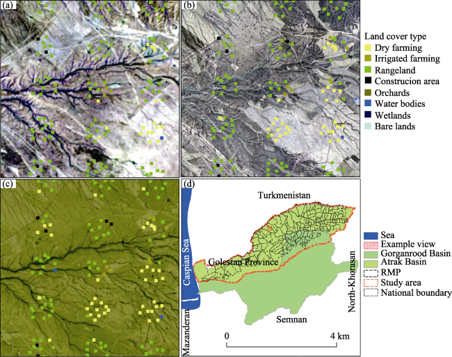
Figure 1 The procedure of GCPs collecting for (a) 1986 on the color composite image of Landsat 5, (b) 2000 on the merged image of Landsat 7, (c) 2015 on the merged image of Landsat 8, and (d) location of the study area and an example view |
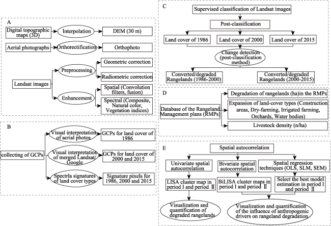
Figure 2 The procedures of visualization and quantification of degraded rangeland: (A) data preprocessing and image enhancement, (B) GCPs and training set selection, (C) image classification and land-cover change detection, (D) creation of a database for Rangeland Management Plans (RMPs), and (E) spatial autocorrelation approaches. |
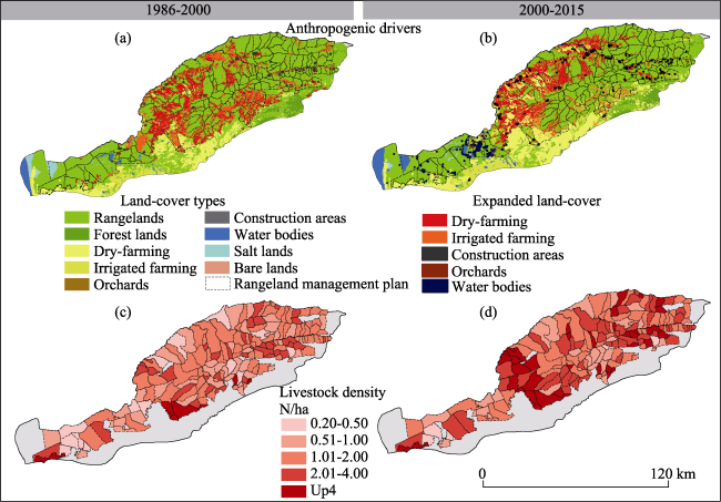
Figure 3 The expansion of anthropogenic land-cover and livestock density from 1986 to 2000 (a, c) and from 2000 to 2015 (b, d) in the RMPs |
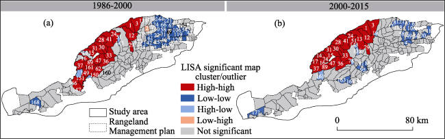
Figure 4 LISA clustering during the period of 1986-2000 (a) and the period of 2000-2015 (b) with p < 0.05 |
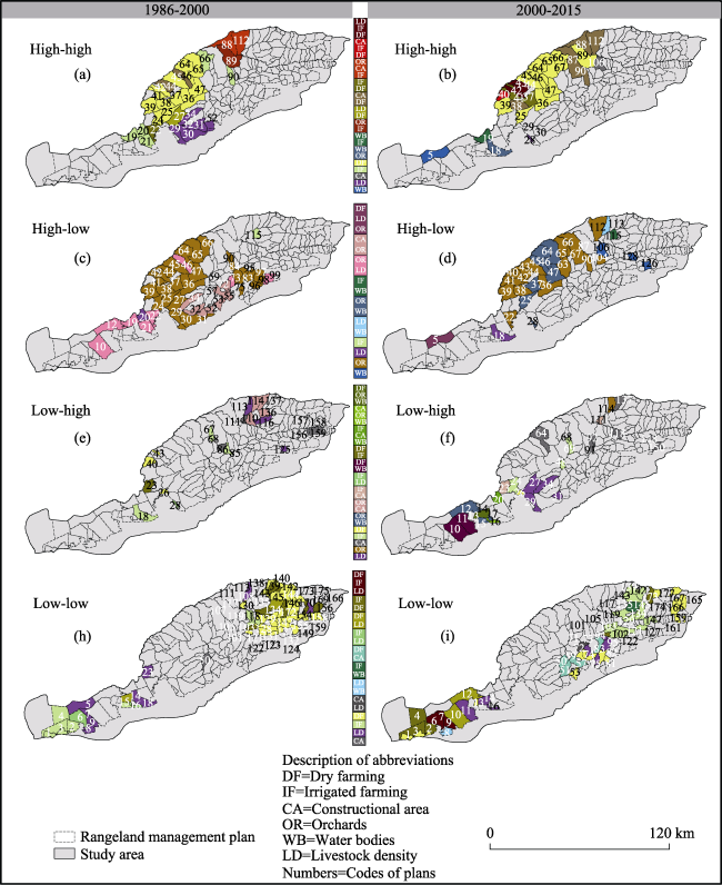
Figure 5 BiLISA clustering showing driving forces (dry-farming, irrigated farming, construction areas, orchards, water bodies and livestock density) influencing degradation of rangelands with four categories of High-High (a, b), High-Low (c, d), Low-High (e, f) and Low-Low (h, I) in the periods of 1986-2000 and 2000-2015 (b) with p < 0.05 |
Table 1 Bivariate local Moran’s I statistics: spatial autocorrelation between degradation of rangelands and expansion of anthropogenic drivers (empirical pseudo significance based on 999 random permutations) |
| 1986-2000 | 2000-2015 | ||||||||
|---|---|---|---|---|---|---|---|---|---|
| Drivers | Local Moran’s I | Cluster/ Outlier | Number of RMPs | Degradation rate (%) | Local Moran’s I | Cluster/ Outlier | Number of RMPs | Degradation rate (%) | |
| Dry-farming (DF) | 0.533*** | High-High | 16 | 22 | 0.509*** | High-High | 22 | 17.31 | |
| Low-Low | 40 | 1.30 | Low-Low | 30 | 0.89 | ||||
| Low-High | 4 | 8.10 | Low-High | 7 | 0.54 | ||||
| High-Low | 0 | 0 | High-Low | 1 | 3.27 | ||||
| Not Significant | 118 | 9 | Not Significant | 118 | 4.04 | ||||
| Irrigated Farming (IF) | 0.200*** | High-High | 9 | 16.92 | 0.157*** | High-High | 7 | 20.77 | |
| Low-Low | 17 | 0.89 | Low-Low | 24 | 0.97 | ||||
| Low-High | 7 | 3.46 | Low-High | 5 | 0.93 | ||||
| High-Low | 1 | 14.38 | High-Low | 2 | 11.64 | ||||
| Not Significant | 144 | 10.67 | Not Significant | 140 | 7.33 | ||||
| Orchards (OR) | -0.00987ns | High-High | 3 | 11.96 | -0.0273ns | High-High | 1 | 13.69 | |
| Low-Low | 0 | 0 | Low-Low | 0 | 0 | ||||
| Low-High | 7 | 1.40 | Low-High | 8 | 0.58 | ||||
| High-Low | 43 | 19.36 | High-Low | 25 | 17.38 | ||||
| Not Significant | 125 | 3.86 | Not Significant | 144 | 2.73 | ||||
| Construction Area (CA) | 0.0754* | High-High | 4 | 14.33 | 0.293*** | High-High | 7 | 17.58 | |
| Low-Low | 1 | 2.03 | Low-Low | 5 | 0.54 | ||||
| Low-High | 10 | 1.65 | Low-High | 10 | 2.25 | ||||
| High-Low | 10 | 17.97 | High-Low | 0 | 0 | ||||
| Not Significant | 153 | 9.86 | Not Significant | 156 | 6.14 | ||||
| Water Body (WB) | - | High-High | - | - | -0.0407ns | High-High | 3 | 7.29 | |
| Low-Low | - | - | Low-Low | 1 | 0.048 | ||||
| Low-High | - | - | Low-High | 9 | 0.82 | ||||
| High-Low | - | - | High-Low | 13 | 13.57 | ||||
| Not Significant | - | - | Not Significant | 152 | 6.34 | ||||
Livestock Density (LD) | 0.005ns | High-High | 7 | 14.47 | 0.0601ns | High-High | 6 | 29.28 | |
| Low-Low | 8 | 2.01 | Low-Low | 15 | 0.58 | ||||
| Low-High | 3 | 15.98 | Low-High | 4 | 0.67 | ||||
| High-Low | 1 | 17.83 | High-Low | 3 | 8.38 | ||||
| Not Significant | 159 | 9.71 | Not Significant | 150 | 7.30 | ||||
Significance levels: ns р-value >0.1; *р-value<0.05; **р-value<0.01; ***р-value<0.001 |
Table 2 Regression analyses of spatial dependencies between degradation rates of rangelands with expansion rates of anthropogenic drivers and livestock density in 1986-2000 |
| Ordinary Least Squares | Spatial Lag | Spatial Error | |||||||
|---|---|---|---|---|---|---|---|---|---|
| Model estimation | Coefficient (β) | t- Statistic | Standard Error | Coefficient (β) | z-Statistic | Standard Error | Coefficient (β) | z-Statistic | Standard Error |
| Constant (β0) | 24.40ns | 1.27 | 19.15 | 14.63ns | 0.751 | 19.49 | 23.353ns | 1.183 | 19.736 |
| Livestock density (x1) | -4.43ns | -0.578 | 7.663 | -6.266ns | 7.599 | -0.825 | -3.579ns | -0.468 | 7.642 |
| Dry-farming (x2) | 0.908*** | 39.008 | .0233 | 0.877*** | 29.543 | 0.029 | 0.905*** | 37.824 | 0.024 |
| Irrigated farming (x3) | 1.004*** | 24.234 | 0.041 | 0.991*** | 24.013 | 0.041 | 1.002*** | 24.121 | 0.041 |
| Orchards (x4) | 0.695ns | 0.598 | 1.162 | 0.606ns | 0.534 | 1.135 | 0.633ns | 0.553 | 1.144 |
| Construction areas (x5) | 1.917ns | 0.837 | 2.291 | 2.083ns | 0.931 | 2.236 | 2.092ns | 0.923 | 2.266 |
| Ƿwy | - | - | - | 0.0502* | 1.611 | 0.031 | - | - | - |
| Lambda (ʎwv) | - | - | - | 0.078ns | 0.775 | 0.100 | |||
| The model fit criteria | Coefficient | Coefficient | Coefficient | ||||||
| AICc | 2339.371 | 2338.643 | 2338.955 | ||||||
| Log likelihood | -1163.685 | -1163.321 | -1163.477 | ||||||
| wi | 0.2789 | 0.3943 | 0.3266 | ||||||
| Ei**** | 1.000 | 1.4139 | 1.1710 | ||||||
Significance levels: ns р-value >0.1; *р-value <0.05; **р-value <0.01; ***р-value <0.001;****Compared with OLS |
Table 3 Regression analyses of spatial dependencies between degradation rates of rangelands with expansion rates of anthropogenic drivers and livestock density in 2000-2015 |
| Ordinary Least Squares | Spatial Lag | Spatial Error | |||||||
|---|---|---|---|---|---|---|---|---|---|
| Model estimation | Coefficient (β) | t- Statistic | Standard Error | Coefficient (β) | z- Statistic | Standard Error | Coefficient (β) | z- Statistic | Standard Error |
| Constant (β0) | -2.004ns | -0.0811 | 24.692 | -8.783ns | -0.355 | 24.755 | -20.536ns | -0.625 | 32.868 |
| Livestock density (x1) | 8.474* | 2.318 | 3.655 | 8.182* | 2.262 | 3.617 | 12.236*** | 3.445 | 3.552 |
| Dry-farming (x2) | 0.879*** | 21.917 | 0.0401 | 0.853*** | 18.298 | 0.047 | 0.878*** | 20.836 | 0.042 |
| Irrigated farming (x3) | -0.162ns | -0.134 | 1.212 | -0.213ns | -0.176 | 1.202 | 1.997* | 1.729 | 1.155 |
| Orchards (x4) | -12.993ns | -0.415 | 31.285 | -12.287ns | -0.402 | 30.571 | -2.805ns | -0.094 | 29.799 |
| Construction areas (x5) | 5.283ns | 0.259 | 20.373 | 6.011ns | 0.302 | 19.908 | 5.674ns | 0.295 | 19.225 |
| Water bodies (x6) | 0.656ns | 0.935 | 0.702 | 0.640ns | 0.933 | 0.687 | -0.220ns | -0.341 | 0.647 |
| ρwy | - | - | - | 0.050 ns | 0.977 | 0.051 | - | - | - |
| Lambda (λwv) | - | - | - | - | - | - | 0.369*** | 4.304 | 0.086 |
| The model fit criteria | Coefficient | Coefficient | Coefficient | ||||||
| AICc | 2503.395 | 2502.560 | 2502.545 | ||||||
| Log likelihood | -1244.281 | -1243.780 | -1243.272 | ||||||
| wi | 0.3202 | 0.4833 | 0.4853 | ||||||
| Ei**** | 1.000 | 1.509 | 1.515 | ||||||
The authors have declared that no competing interests exist.
| [1] |
|
| [2] |
|
| [3] |
|
| [4] |
|
| [5] |
|
| [6] |
|
| [7] |
|
| [8] |
|
| [9] |
|
| [10] |
|
| [11] |
|
| [12] |
|
| [13] |
|
| [14] |
|
| [15] |
|
| [16] |
|
| [17] |
|
| [18] |
|
| [19] |
|
| [20] |
|
| [21] |
|
| [22] |
|
| [23] |
|
| [24] |
|
| [25] |
DEI, 2003. Iran’s Initial National Communication to UNFCCC. Department of Environment and United Nation Department Programme: Tehran, 206pp.
|
| [26] |
DEI, 2010. Iran second national communication to UNFCCC. National Climate Change Office of Iran at the Department of Environment: Tehran, 205pp.
|
| [27] |
|
| [28] |
|
| [29] |
|
| [30] |
|
| [31] |
|
| [32] |
|
| [33] |
|
| [34] |
|
| [35] |
|
| [36] |
|
| [37] |
|
| [38] |
|
| [39] |
|
| [40] |
|
| [41] |
|
| [42] |
|
| [43] |
|
| [44] |
|
| [45] |
|
| [46] |
|
| [47] |
|
| [48] |
|
| [49] |
|
| [50] |
|
| [51] |
|
| [52] |
|
| [53] |
|
| [54] |
|
| [55] |
|
| [56] |
|
| [57] |
|
| [58] |
|
| [59] |
|
| [60] |
|
| [61] |
|
| [62] |
|
| [63] |
|
| [64] |
|
| [65] |
The Presidential Deputy Office of Strategic Planning and Control(PDOSPC), 2011. Law for the Fifth Development Plan of the Islamic Republic of Iran (IR038). Retrieved from .
|
| [66] |
|
| [67] |
|
| [68] |
|
| [69] |
|
| [70] |
|
| [71] |
|
| [72] |
|
| [73] |
|
/
| 〈 |
|
〉 |