Research Articles

Measurement of vegetation parameters and error analysis based on Monte Carlo method

  • LIANG Boyi , 1 ,
  • LIU Suhong , 2, *
Expand
  • 1. College of Urban and Environment Sciences, Peking University, Beijing 100871, China
  • 2. Faculty of Geography, Beijing Normal University, Beijing 100875, China
*Corresponding author: Liu Shihong, E-mail:

Author: Liang Boyi, E-mail:

Received date: 2017-06-30

  Accepted date: 2017-12-08

  Online published: 2018-06-20

Supported by

National Natural Science Foundation of China, No.41171262

Copyright

Journal of Geographical Sciences, All Rights Reserved

Abstract

In this paper we bring up a Monte Carlo theory based method to measure the ground vegetation parameters, and make quantitative description of the error. The leaf area index is used as the example in the study. Its mean and variance stability at different scales or in different time is verified using both the computer simulation and the statistics of remotely sensed images. And the error of Monte Carlo sampling method is analyzed based on the normal distribution theory and the central-limit theorem. The results show that the variance of leaf area index in the same area is stable at certain scales or in the same time of different years. The difference between experimental results and theoretical ones is small. The significance of this study is to establish a measurement procedure of ground vegetation parameters with an error control system.

Cite this article

LIANG Boyi , LIU Suhong . Measurement of vegetation parameters and error analysis based on Monte Carlo method[J]. Journal of Geographical Sciences, 2018 , 28(6) : 819 -832 . DOI: 10.1007/s11442-018-1507-8

1 Introduction

Being one of the main components of the terrestrial biosphere, vegetation accounts for about 50% of the earth’s surface area, and it plays an important role in the earth system by making contribution for atmospheric controlling, water purification, climate regulation, soil and water conservation and so on (Sato et al., 1989; Lean and Rowntree, 1993; Weiss and Baret, 1999; Raich and Tufekciogul, 2000; Ceccato et al., 2001). The vegetation parameters, such as leaf area index (LAI), fractional vegetation coverage (FVC), are key agronomic and ecological parameters, which are of great importance to the study of hydrology, ecology and global change (Fitzgerald et al., 2005; Liang et al., 2015; Barton and North, 2001; Colombo et al., 2003).
The measurement method of vegetation parameters mainly includes ground-based measurement and remote sensing inversion (Ding et al., 2007; Liu et al., 2014; Phillips et al., 1998; González et al., 2008). Since the 1990s, the use of remote sensing data for long time series and large-scale vegetation parameters inversion has become more and more common (Gao 1996; Singh, 1989; Lefsky et al., 2002; Yu et al., 2006; Valentini et al., 2000; Xu et al., 2013). However, due to the limitations of remote sensing technology, there is a lot of uncertainty in this method (Richey et al., 2002; Benz et al., 2004). Therefore, it is necessary to carry out the ground verification work while retrieving vegetation parameters by using remote sensing data in order to improve the reliability of the results (Chen and Cihlar, 1995; Tan, 2016; Shao et al., 2017). Taking LAI as an example, the ground measurement method mainly includes direct measurement method, digital photography method or using other instruments. Instruments which are frequently used include LAI-2000, Sunfleck Ceptometer, TRAC (Bréda, 2003). Under normal circumstances, people often use system sampling method to select some parts of the study region as the samples, and take the average value of samples as the result of the whole study area, which may result in some error. For the assessment of error, people would normally use their own study area for statistical analysis with no identical standard. So there is still a lack of universal system of error assessment (Manies and Mladenoff, 2000; Mehner et al., 2004).
Monte Carlo method is also called statistical simulation method. Unlike the general deterministic model, the errors need to be analyzed by probabilistic methods (Evensen, 1994; Hastings, 1970; Koehler et al., 2009). Ground-based measurement of vegetation parameters mentioned above is one kind of Monte Carlo random sampling method. In this paper, the variance stability of LAI at different scales and in different time periods was verified using both the computer simulation (micro perspective) and the remote sensing data (macro perspective). The experiment first calculated the theoretical error distribution, and then verified the consistency between real error and theoretical one. By selecting different sampling quantities to measure the vegetation parameters under different vegetation conditions and precision requirements in the study area, we solved the problem of error analysis. Besides, this method was suitable for any scales.

2 Data and methods

The vegetation scenarios with three different LAI levels were simulated by computer program. The mean and variance of LAI in each scene were calculated and the frequency curve was generated. The variance stability was observed at different scales. GLASS LAI data was used for verification of variance stability index in different time. In the study, we selected the products for 10 years from 2004 to 2013, taking the 201st day of the year (DOY) as an example, and choosing the three research areas according to their LAI levels.

2.1 Computer simulation

Based on fractal tree theory (Frontier, 1987; Lin and Sarabandi, 1999; Weibel, 1999), three scenarios with different vegetation levels (high, medium, low) were randomly generated by computer program. The tree height obeys normal distribution while the position of trees obeys Poisson distribution.
Here, we defined the concept of two-dimensional LAI: first make the side projection of a three-dimensional vegetation scene to the two-dimensional plane, and the sum length of leaves in unit horizontal length was described as two-dimensional LAI. We selected different length as sampling scales (1, 2, 4, 8, 16, 32, 64 and 128, unit: pixel, defined as Δx) and calculated the mean, variance and frequency curves of the LAI at different scales under the three scenarios (Figure 1).
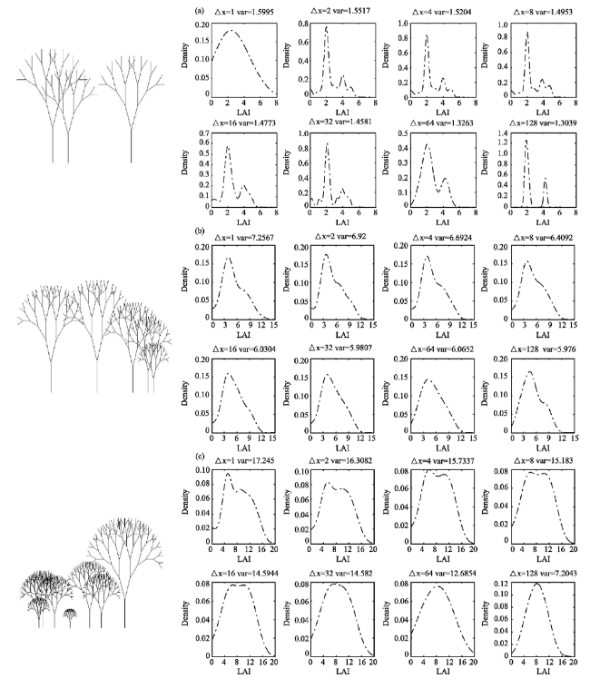
Figure 1 Vegetation scenarios simulated by computer and their leaf area index frequency curves (a. low level; b. median level; c. high level)
In low level scenario, frequency curve of LAI at different scales showed a high consistency except for the circumstances when Δx was 1,128 or 256. This was because the horizontal length of the whole scene was 512 pixels, so when Δx was equal to 64 or 128, the number of samples was too small, which was 8 or 4 respectively, resulting in the relative abnormalities of the curve. For the median level scenario, the frequency curves at different scales were more similar to those in low level scene. All curves increased at first and then went down from their peaks. It was not difficult to find that in the computer simulation cases, the frequency curves were irregular regardless of the level of LAI, which did not belong to any kind of common distribution.
Figure 2 showed the variance scatter plot at different scales in computer simulation cases (low level, median level and high level from the bottom to the top). The variance of LAI decreased with the increase of sampling scale. When the sampling scale was 2, 4, 8, 16, 32 (pixels), the curve was relatively smooth. When the sampling scale rose to 64 and 128 (pixels), the variance began to degrade significantly, especially for the low level and high level cases.
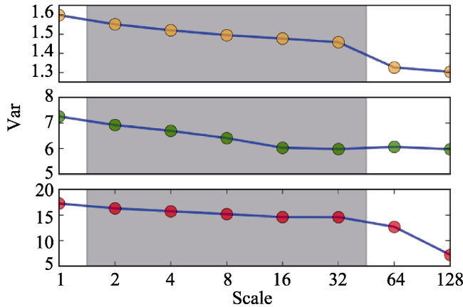
Figure 2 LAI variations in computer simulation

2.2 Remote sensing data

Similar to the cases in the computer simulation, three areas (low, median, high level of LAI) were selected in GLASS LAI images (Figure 3, produced by Arcgis 10.0). The three regions were located in Amazon rainforest (55.075°W-70.25°W, 14.925°S-0.025°N), boreal forest in North Asia (94.975°E-109.925°E, 60.075°N-75.025°N) and Northwest America (95.075°W-110.025°W, 30.075°N-45.025°N) respectively. The mean, variance and frequency curves of LAI in different years were calculated as shown in Figure 4.
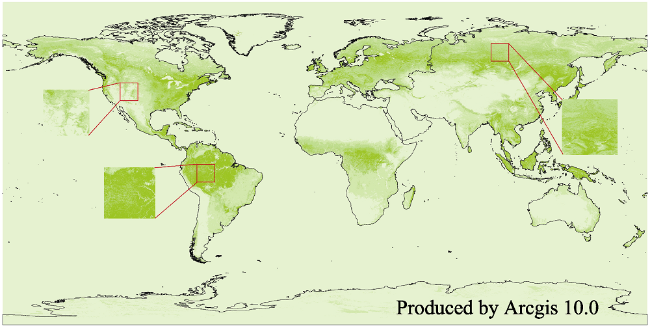
Figure 3 GLASS LAI of the study area
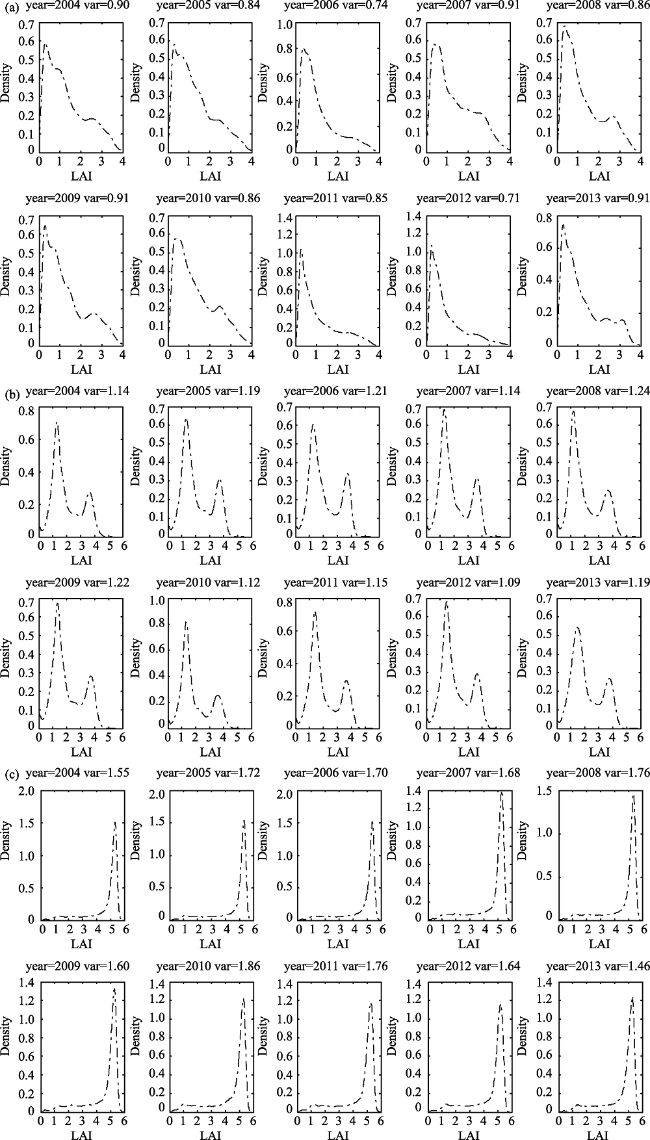
Figure 4 Frequency curves of GLASS LAI (a. low level. b. median level. c. high level)
The frequency curves of LAI in the three study regions had different random shapes. The curves have only one “peak” in the high and low level regions, while it was “bimodal” in the median level area. From 2004 to 2013, the variances of LAI in the low, median and high level region ranged from 0.71 to 0.91, from 1.09 to 1.24 and from 1.46 to 1.84 respectively. In the ten-year time series, variance kept relatively stable.

2.3 Analysis of error probability

For a random variable x that obeys normal distribution, the probability density function is (Stein, 1981; Epanechnikov, 1969):
$f(x)=\frac{1}{\sqrt{2\pi }\sigma }{{e}^{-\frac{{{(x-\mu )}^{2}}}{2{{\sigma }^{2}}}}},-\infty <x<+\infty $
where μ and σ are both constant, representing the mean and standard deviation respectively.
And if the variable x obeys normal distribution, its distribution function is:
$F(x)=\frac{1}{\sqrt{2\pi }\sigma }\int_{-\infty }^{x}{{{e}^{-\frac{{{(x-\mu )}^{2}}}{2{{\sigma }^{2}}}}}}dx,-\infty <x<+\infty $
And the probability of variable X between x1 and x2 is:
$P({{x}_{1}},{{x}_{2}})=F({{x}_{2}})-F({{x}_{1}})$
According to the Lindeberg-Levi theorem (independent distribution center limit theorem) (Ditlevsen et al., 1996; Nishiyama, 2001; Li and Ullha, 1998), if ξ1, ξ2, ..., ξn, ... are a series of independent identically distributed random variables, the expect i = μ, the variance i = σ2> 0, i = 1,2, ..., then:
$\underset{n-\infty }{\mathop{lim}}\,P\left\{ \frac{\sum\limits_{i=1}^{n}{{{\xi }_{i}}-n\mu }}{\sqrt{n}\sigma }\le x \right\}=\frac{1}{\sqrt{2\pi }}\int_{-\infty }^{x}{{{e}^{-\frac{{{t}^{2}}}{2}}}dt}={{\Phi }_{0}}(x), $
${{Y}_{n}}=\frac{\sum\limits_{i=1}^{n}{{{\xi }_{i}}-n\mu }}{\sqrt{n}\sigma }\tilde{\ }{{F}_{n}}(x), \underset{n\to \infty }{\mathop{lim}}\,P({{Y}_{n}}\le x)={{\Phi }_{0}}(x), \ \underset{n\to \infty }{\mathop{lim}}\,F(x)={{\Phi }_{0}}(x), $${{Y}_{n}}=\frac{\sum\limits_{i=1}^{n}{{{\xi }_{i}}}-n\mu }{\sqrt{n}\sigma }\tilde{\ }N(0,1),$ $\sum\limits_{i=1}^{n}{{{\xi }_{i}}}\tilde{\ }N(n\mu ,n{{\sigma }^{2}}),$$\frac{1}{n}\sum\limits_{i=1}^{n}{{{\xi }_{i}}}\tilde{\ }N\left( \mu ,\frac{{{\sigma }^{2}}}{n} \right)$
The theorem states that when we use a sampling method for measuring a variable with an independent identity (μ is the mean, σ is the standard deviation), the mean value obeys a normal distribution (the mean is μ, the variance is σ2/n) theoretically as long as n is large enough (generally greater than 30), regardless of the distribution of the source data. We applied this theory to the LAI sampling method. Accordingly, when the sampling quantity (number of sampling points or pixels) is large enough, the mean should also obey normal distribution. In addition, the theory also shows that mean value distribution of sampling method is only related to sampling quantity, and has nothing to do with the measurement range. Therefore, we can avoid the scale effect under the hypothesis that the measured results for each time are true values. In this paper, we used the distribution function of normal distribution to calculate theoretical probability of sampling mean value located in different error intervals, establishing the error evaluation system about the sampling method for LAI.
According to the theory described above, a set of ground vegetation parameter measurement processes containing quantitative description of error could be established. We still take LAI as an example. The measurement steps were as follows:
(1) Select the study area on earth. The area could be any size, and we did not need to consider the distribution of vegetation or other geographical parameters in it.
(2) Calculate the frequency histogram of LAI in the entire study area by remote sensing (aerial or aerospace) images, at as many scales as possible. We assumed that the value retrieved by remote sensing images at different scales is true.
(3) Measure LAI in the study area at different scales (from minimum to maximum) or in different time and calculate the variations of them. Through this process, we obtained only one measurement result without variation at the maximum scale (whole area) .The minimum scale referred to the smallest unit which could be achieved technically, such as the highest spatial resolution in remote sensing image. Other scales between the maximum and minimum ranges were regarded as intermediate scales, and the variance could be stable within certain range. Next, optimal scales were selected artificially according to the requirement of measurement error. Finally, the mean variance at optimal scales or in different periods of time was regarded as the variance of the whole study area.
(4) Use normal distribution theory and the Lindbergh-Levi theorem to calculate the error distribution by using different random sampling quantities. The sampling quantity (which can be sampled at any scale) is determined according to the measurement cost and accuracy requirements. When the error requirement is high, we need more sampling points to make the variance of the mean value smaller and the result closer to the true value of LAI.
(5) Compare the error results deduced from the theory with the real measurement to verify the reliability of error probability distribution.

3 Result and discussion

3.1 Verification of normal distribution

The six scenarios of computer simulation and GLASS LAI were measured by sampling method. The number of samples was selected as 30, 50, 70, 100, 150, 200, 300 and 500 respectively. For the computer simulation scenario, the sampling unit was the width of one pixel; GLASS LAI was sampled by unit of one pixel. We used computer program to simulate the measurement process of each sampling quantity for 1000 times, and get 1000 sets of mean value. Then we tested the normal distribution of these results shown in Figure 5 with the abscissa being the mean value of LAI under different sampling quantities. In this diagram, the closer the points were to diagonal, the better they obeyed normal distribution. It could be seen that the mean values of all six study areas were close to the normal distribution regardless of sampling quantities. We can find that when the points were centralized in the middle area, the shape was more close to the normal distribution. In contrast, points away from middle had irregular shape of distribution, which was related to the number of simulation cycles.
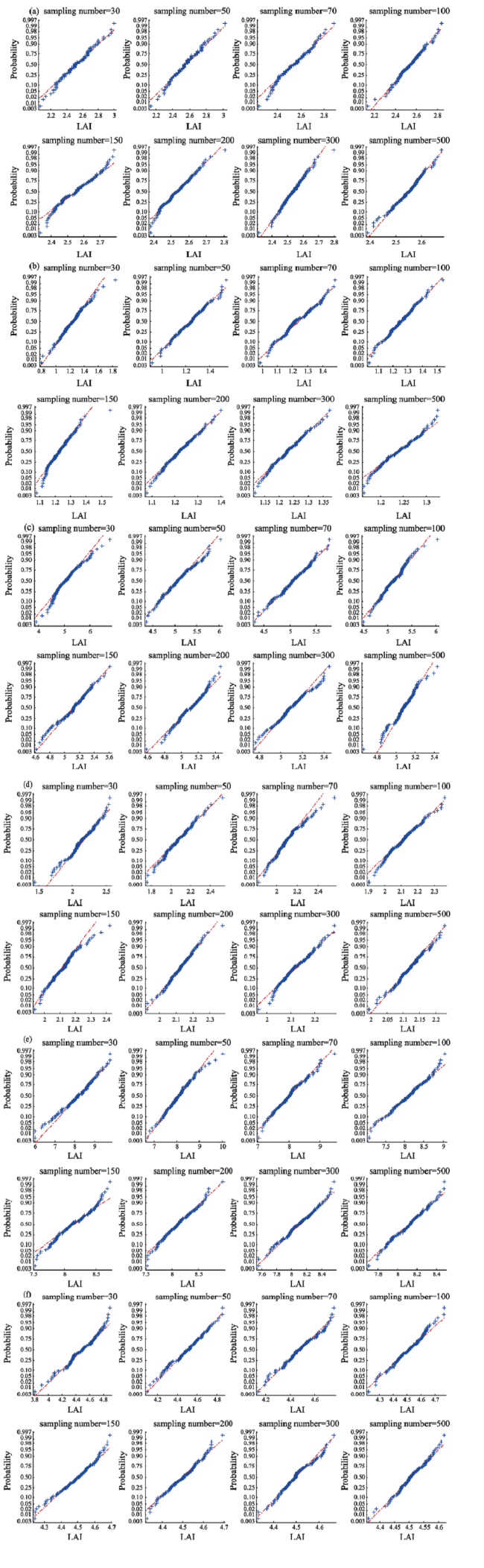
Figure 5 Verification of normal distribution (a. low level of computer simulation; b. low level of GLASS LAI; c. median level of computer simulation; d. median level of GLASS LAI; e. high level of computer simulation; f. high level of GLASS LAI)

3.2 Verification of mean and variation

For the three vegetation scenarios simulated by computer program, the variance of whole scene was taken as the mean variation at the six median scales, while the variance of the three GLASS LAI regions was taken as the mean value of variation in ten years (from 2004 to 2013). The theoretical value of mean LAI and its variation in three scenarios and three study areas under different sampling quantities were calculated by using the Lindbergh - Levi theorem. Then we calculated the real mean LAI and variance for 1000 times by computer simulation, and compared the results with the theoretical ones (Table 1).
Table 1 Verification of mean and variation
Sampling quantity 30 50 70 100 150 200 300 500
Low level Computer simulation Variation Theoretical value 0.049 0.029 0.021 0.015 0.010 0.007 0.005 0.003
Real value 0.056 0.032 0.022 0.016 0.011 0.008 0.006 0.003
Mean Theoretical value 2.535 2.535 2.535 2.535 2.535 2.535 2.535 2.535
Real value 2.531 2.546 2.541 2.536 2.537 2.534 2.540 2.537
GLASS LAI Variation Theoretical value 0.028 0.017 0.012 0.008 0.006 0.004 0.003 0.002
Real value 0.031 0.018 0.013 0.009 0.006 0.005 0.003 0.002
Mean Theoretical value 1.234 1.234 1.234 1.234 1.234 1.234 1.234 1.234
Real value 1.243 1.240 1.228 1.231 1.230 1.233 1.231 1.231
Median level Computer simulation Variation Theoretical value 0.212 0.127 0.091 0.064 0.042 0.032 0.021 0.013
Real value 0.245 0.153 0.105 0.076 0.047 0.035 0.024 0.015
Mean Theoretical value 5.086 5.086 5.086 5.086 5.086 5.086 5.086 5.086
Real value 5.073 5.091 5.097 5.079 5.083 5.084 5.087 5.091
GLASS LAI Variation Theoretical value 0.039 0.023 0.017 0.012 0.008 0.006 0.004 0.002
Real value 0.038 0.024 0.016 0.011 0.008 0.006 0.004 0.002
Mean Theoretical value 2.115 2.115 2.115 2.115 2.115 2.115 2.115 2.115
Real value 2.099 2.122 2.118 2.117 2.113 2.115 2.115 2.115
High level Computer simulation Variation Theoretical value 0.495 0.297 0.212 0.148 0.099 0.074 0.049 0.030
Real value 0.532 0.352 0.270 0.176 0.122 0.085 0.054 0.035
Mean Theoretical value 8.086 8.086 8.086 8.086 8.086 8.086 8.086 8.086
Real value 8.089 8.096 8.087 8.081 8.103 8.090 8.081 8.096
GLASS LAI Variation Theoretical value 0.056 0.033 0.024 0.017 0.011 0.008 0.006 0.003
Real value 0.047 0.030 0.020 0.015 0.009 0.007 0.005 0.003
Mean Theoretical value 4.498 4.498 4.498 4.498 4.498 4.498 4.498 4.498
Real value 4.493 4.498 4.501 4.503 4.504 4.505 4.502 4.500
The difference between real and theoretical value of variation was small in general. In the computer simulation cases, the maximum error occurred when sampling quantity was 30, and the maximum errors in low, medium and high level scenes were 0.007, 0.033 and 0.037 respectively. As the LAI level increased, the error became smaller gradually. The variance error of GLASS LAI was similar, the maximum error occurred identically when the sampling quantity was 30, and the maximum errors in low, medium and high level scenes were 0.003, 0.001 and 0.009 respectively. The result of the mean was compliant to the theorem, that was, as the number of sampling points increased, the sampling mean became more and more convergent to the theoretical value.

3.3 Verification of probability error

In this section, we took high-level area simulated by the computer program as an example. First, we calculated theoretical error distribution by different sampling quantities, and then conducted the verification of theoretical error.
Figure 6 showed the quantitative relationship among sampling quantity, ratio of error and mean value (error interval), and frequency of the sampling mean. It could be seen from the figure that when the error interval was small, the mean value ratio increased gradually in the error interval with the increase of the sampling quantity. When the error interval was large, the proportion of the mean in the error interval reduced as the sampling quantity increased. Figure 6b stood for the vertical projection of Figure 6a above which showed clearly that roughly 4% error is the dividing line. When the error interval was less than 4%, the sampling mean frequency increased with the increase of sampling quantity and if error interval was greater than 4%, the sampling mean frequency decreased as sampling quantity increased. Namely, with the increase of sampling quantities, the sampling mean distribution was getting closer to the theoretical one, and the overall error was getting smaller.
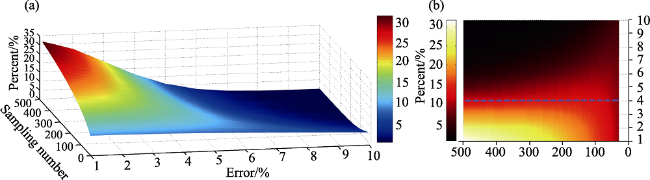
Figure 6 Error distribution (a. three dimensional graph; b. orthographic projection)
The error distribution of LAI sampling mean value in high level area under different sampling quantities was simulated by computer program. Each pie chart showed the probability of the mean result error in different intervals by each sampling quantity. The middle region represented the result of the simulation (regarded as the real value), and the peripheral number represented the theoretical value. Table 2 showed the absolute value of the difference between the theoretical and real ratio in different error intervals.
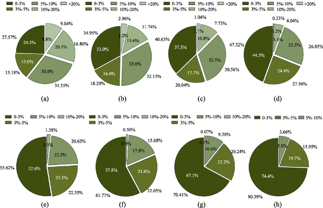
Table 2 Statistics of error distribution
Sampling quantity 0-3% 3%-5% 5%-10% 10%-20% >20% Average
30 3.07% 0.18% 0.75% 3.24% 0.76% 1.60%
50 1.95% 1.60% 1.45% 1.86% 0.24% 1.42%
70 3.33% 2.34% 1.94% 3.07% 0.66% 2.27%
100 2.82% 2.84% 1.35% 1.36% 0.03% 1.68%
150 3.20% 0.95% 1.59% 0.52% 1.57%
200 3.97% 1.55% 2.12% 0.30% 1.99%
300 3.31% 1.96% 1.32% 0.03% 1.66%
500 5.99% 3.75% 2.24% 3.99%
Figure 7 Error distribution under different sampling quantities (a. 30; b. 50; c. 70; d. 100; e. 150; f. 200; g. 300; h. 500)
Table 2 showed that the difference between the real value and theoretical one was quite small. In addition, with the increase of sampling quantity, the proportion of those small error intervals gradually increased, while that of larger error interval gradually decreased. If the sampling quantity was more than 150, the proportion with error intervals being greater than 20% was too small to be counted; similarly, if the sampling quantity was more than 500, there were only three kinds of difference in error intervals. Besides, when the sampling quantity was 30, the largest difference between theoretical and real ratio was 3.24%, being located in the interval of 10%-20%; if the sampling quantities were 50, 70, 150, 200, 300, 500 respectively, the largest difference between theoretical and real ratio were 1.95%, 3.33%, 3.02%, 3.97%, 3.31% and 5.99%, being located in the interval of 0%-3%; and when the sampling quantity was 100, the largest difference between theoretical and real ratio was 2.84%, being located in the interval of 3%-5%. This proved the correctness of the previous theoretical error distribution, and showed that using the mean variance at intermediate scales or multiples years as the variance of whole study area had some rationality.

4 Conclusions

This paper proposed a vegetation parameter measurement method based on Monte Carlo's theory which included a quantitative error assessment system. The method solves the problem that the error cannot be evaluated when the ground parameters are measured in the past. The complete steps of random sampling measurement of vegetation parameters have high feasibility. This paper has three important conclusions:
(1) When the study area is fixed, the variance of the vegetation parameters at intermediate scales or at the same time of different years has a characteristic of stability, we can take the average value as variance of the whole study area.
(2) According to the normal distribution theory and the Lindbergh-Levi theorem, we can deduce the distribution of the mean of the samples under different sampling quantities, and further calculate the theoretical probability of the mean in different error intervals.
(3) It is found that the error distribution is highly consistent with the theoretical one by simulating the process of measurement, which shows the rationality of error control and the feasibility of sampling method under the error evaluation system. The controlling of the error not only allows the surveyor to have a quantitative expectation for the measurement results, but also makes the allocation of measurement work more rational, in accordance with the requirement of accuracy. We can select the most appropriate sampling quantity of measurement and reduce the cost, as well as improving work efficiency.

5 Discussion

The method proposed in this paper is not only applicable to the ground measurement of vegetation parameters, but also practical to other geometric parameters in wide regions. When distributing the layout of the measurement station, the variance characteristics of the geographical parameters in the area are ought to be taken into account. For example, in areas where the parameter differentiation is obvious, the number of measurement should be increased and if the area has high degree of parameter uniformity, we can establish less measurement stations for saving cost. The geographical parameters mentioned include not only the ground parameters but also the various variables in the atmosphere which has this kind of stability. This idea of quantitative sampling method has great value for further study in the future.

The authors have declared that no competing interests exist.

[1]
Barton C V M, North P R J, 2001. Remote sensing of canopy light use efficiency using the photochemical reflectance index: Model and sensitivity analysis.Remote Sensing of Environment, 78: 264-273.

DOI

[2]
Benz U C, Hofmann P, Willhauck G, 2004. Multi-resolution, object-oriented fuzzy analysis of remote sensing data for GIS-ready information.ISPRS Journal of Photogrammetry and Remote Sensing, 58: 239-258.Remote sensing from airborne and spaceborne platforms provides valuable data for mapping, environmental monitoring, disaster management and civil and military intelligence. However, to explore the full value of these data, the appropriate information has to be extracted and presented in standard format to import it into geo-information systems and thus allow efficient decision processes. The object-oriented approach can contribute to powerful automatic and semi-automatic analysis for most remote sensing applications. Synergetic use to pixel-based or statistical signal processing methods explores the rich information contents. Here, we explain principal strategies of object-oriented analysis, discuss how the combination with fuzzy methods allows implementing expert knowledge and describe a representative example for the proposed workflow from remote sensing imagery to GIS. The strategies are demonstrated using the first object-oriented image analysis software on the market, eCognition, which provides an appropriate link between remote sensing imagery and GIS.

DOI

[3]
Bréda N J J, 2003. Ground-based measurements of leaf area index: A review of methods, instruments and current controversies.Journal of Experimental Botany, 54: 2403-2417.Abstract Leaf area index (LAI) is the total one-sided area of leaf tissue per unit ground surface area. It is a key parameter in ecophysiology, especially for scaling up the gas exchange from leaf to canopy level. It characterizes the canopy-atmosphere interface, where most of the energy fluxes exchange. It is also one of the most difficult to quantify properly, owing to large spatial and temporal variability. Many methods have been developed to quantify LAI from the ground and some of them are also suitable for describing other structural parameters of the canopy. This paper reviews the direct and indirect methods, the required instruments, their advantages, disadvantages and accuracy of the results. Analysis of the literature shows that most cross-validations between direct and indirect methods have pointed to a significant underestimation of LAI with the latter techniques, especially in forest stands. The two main causes for the discrepancy, clumping and contribution of stem and branches, are discussed and some recent theoretical or technical solutions are presented as potential improvements to reduce bias or discrepancies. The accuracy, sampling strategy and spatial validity of the LAI measurements have to be assessed for quality assurance of both the measurement and the modelling purposes of all the LAI-dependent ecophysiological and biophysical processes of canopies.

DOI PMID

[4]
Ceccato P, Flasse S, Tarantola S, 2001. Detecting vegetation leaf water content using reflectance in the optical domain.Remote Sensing of Environment, 77: 22-33.This paper outlines the first part of a series of research studies to investigate the potential and approaches for using optical remote sensing to assess vegetation water content. It first analyzes why most methods used as approximations of vegetation water content (such as vegetation stress indices, estimation of degree of curing and chlorophyll content) are not suitable for retrieving water content at leaf level. It then documents the physical basis supporting the use of remote sensing to directly detect vegetation water content in terms of Equivalent Water Thickness (EWT) at leaf level. Using laboratory measurements, the radiative transfer model PROSPECT and a sensitivity analysis, it shows that shortwave infrared (SWIR) is sensitive to EWT but cannot be used alone to retrieve EWT because two other leaf parameters (internal structure and dry matter) also influence leaf reflectance in the SWIR. A combination of SWIR and NIR (only influenced by these two parameters) is necessary to retrieve EWT at leaf level. These results set the basis towards establishing operational techniques for the retrieval of EWT at top-of-canopy and top-of-atmospheric levels.

DOI

[5]
Chen J M, Cihlar J, 1995. Plant canopy gap-size analysis theory for improving optical measurements of leaf-area index.Applied Optics, 34: 6211-6222.Abstract Optical instruments currently available for measuring the leaf-area index (LAI) of a plant canopy all utilize only the canopy gap-fraction information. These instruments include the Li-Cor LAI-2000 Plant Canopy Analyzer, Decagon, and Demon. The advantages of utilizing both the canopy gap-fraction and gap-size information are shown. For the purpose of measuring the canopy gap size, a prototype sunfleck-LAI instrument named Tracing Radiation and Architecture of Canopies (TRAC), has been developed and tested in two pure conifer plantations, red pine (Pinus resinosa Ait.) and jack pine (Pinus banksiana Lamb). A new gap-size-analysis theory is presented to quantify the effect of canopy architecture on optical measurements of LAI based on the gap-fraction principle. The theory is an improvement on that of Lang and Xiang [Agric. For. Meteorol. 37, 229 (1986)]. In principle, this theory can be used for any heterogeneous canopies.

DOI PMID

[6]
Colombo R, Bellingeri D, Fasolini D, 2003. Retrieval of leaf area index in different vegetation types using high resolution satellite data.Remote Sensing of Environment, 86: 120-131.With the successful launch of the IKONOS satellite, very high geometric resolution imagery is within reach of civilian users. In the 1-m spatial resolution images acquired by the IKONOS satellite, details of buildings, individual trees, and vegetation structural variations are detectable. The visibility of such details opens up many new applications, which require the use of geometrical information contained in the images. This paper presents an application in which spectral and textural information is used for mapping the leaf area index (LAI) of different vegetation types. This study includes the estimation of LAI by different spectral vegetation indices (SVIs) combined with image textural information and geostatistical parameters derived from high resolution satellite data. It is shown that the relationships between spectral vegetation indices and biophysical parameters should be developed separately for each vegetation type, and that the combination of the texture indices and vegetation indices results in an improved fit of the regression equation for most vegetation types when compared with one derived from SVIs alone. High within-field spatial variability was found in LAI, suggesting that high resolution mapping of LAI may be relevant to the introduction of precision farming techniques in the agricultural management strategies of the investigated area.

DOI

[7]
Ding M J, Zhang Yili, Liu Linshan.et al, 2007. The relationship between NDVI and precipitation on the Tibetan Plateau.Journal of Geographical Sciences, 17(3): 259-268.The temporal and spatial changes of NDVI on the Tibetan Plateau , as well as the relationship between NDVI and precipitation, were discussed in this paper, by using 8-km resolution multi-temporal NOAA AVHRR-NDVI data from 1982 to 1999. Monthly maximum NDVI and monthly rainfall were used to analyze the seasonal changes, and annual maximum NDVI, annual effective precipitation and growing season precipitation (from April to August) were used to discuss the interannual changes. The dynamic change of NDVI and the correlation coefficients between NDVI and rainfall were computed for each pixel. The results are as follows: (1) The NDVI reached the peak in growing season (from July to September) on the Tibetan Plateau . In the northern and western parts of the plateau, the growing season was very short (about two or three months); but in the southern, vegetation grew almost all the year round. The correlation of monthly maximum NDVI and monthly rainfall varied in different areas. It was weak in the western, northern and southern parts, but strong in the central and eastern parts. (2) The spatial distribution of NDVI interannual dynamic change was different too. The increase areas were mainly distributed in southern Tibet montane shrub-steppe zone, western part of western Sichuan-eastern Tibet montane coniferous forest zone, western part of northern slopes of Kunlun montane desert zone and southeastern part of southern slopes of Himalaya montane evergreen broad-leaved forest zone; the decrease areas were mainly distributed in the Qaidam montane desert zone, the western and northern parts of eastern Qinghai-Qilian montane steppe zone, southern Qinghai high cold meadow steppe zone and Ngari montane desert-steppe and desert zone. The spatial distribution of correlation coefficient between annual effective rainfall and annual maximum NDVI was similar to the growing season rainfall and annual maximum NDVI, and there was good relationship between NDVI and rainfall in the meadow and grassland with medium vegetation cover, and the effect of rainfall on vegetation was small in the forest and desert area.

DOI

[8]
Ditlevsen O, Mohr G, Hoffmeyer P, 1996. Integration of non-Gaussian fields.Probabilistic Engineering Mechanics, 11: 15-23.The limitations of the validity of the central limit theorem argument as applied to definite integrals of non-Gaussian random fields are empirically explored by way of examples. The purpose is to investigate in specific cases whether the asymptotic convergence to the Gaussian distribution is fast enough to justify that it is sufficiently accurate for the applications to shortcut the problem and just assume that the distribution of the relevant stochastic integral is Gaussian. An earlier published example exhibiting this problem concerns silo pressure fields. [Ditlevsen, O., Christensen, C. and Randrup-Thomsen, S. Reliability of silo ring under lognormal stochastic pressure using stochastic interpolation. Proc. IUTAM Symp., Probabilistic Structural Mechanics: Advances in Structural Reliability Methods, San Antonio, TX, USA, June 1993 (eds.: P. D. Spanos & Y.-T. Wu) pp. 134-162. Springer, Berlin, 1994]The numerical technique applied to obtain approximate information about the distribution of the integral is based on a recursive application of Winterstein approximations (moment fitted linear combinations of Hermite polynomials of standard Gaussian variables). The method uses the very long exact formulas for the 3rd and 4th moments of any linear combination of two correlated four-term Winterstein approximations. These formulas are derived by computerized symbol manipulations. Some of the results are compared with some special exact results for sums of Winterstein approximations. [Mohr, G. & Ditlevsen, O. Partial summations of stationary sequences of Winterstein approximations. Prob. Engng Mech. 11 (1996) 25-30.]For decreasing correlation extension including negative correlation, problems of increasing sensitivity to the recursive approximations show up. For practical use of the method, it may therefore, in special situations with negative correlation, be necessary to introduce numerical integration checks or simulation checks of the results.

DOI

[9]
Epanechnikov V A, 1969. Non-parametric estimation of a multivariate probability density.Theory of Probability & Its Applications, 14: 153-158.

[10]
Evensen G, 1994. Sequential data assimilation with a nonlinear quasi-geostrophic model using Monte Carlo methods to forecast error statistics.Journal of Geophysical Research: Oceans, 99: 10143-10162.

[11]
Fitzgerald G J, Pinter P J, Hunsaker D J, 2005. Multiple shadow fractions in spectral mixture analysis of a cotton canopy.Remote Sensing of Environment, 97: 526-539.Shadows are being used more frequently to estimate plant canopy biophysical characteristics. Typically, a zero value is assumed or a threshold value is derived from histogram analysis of imagery to determine the shadow endmember (EM). Here, two distinct shadow EMs were measured in situ for use in spectral mixture analysis of a cotton canopy on five dates in 2003. The four EMs used in the analysis were: sunlit green leaf, sunlit dry soil, self-shadowed leaf, shadowed dry soil. This 4-EM model was compared to a 3-EM model where a zero-value shade EM was used for unmixing with the two sunlit EMs. Multiple endmember spectral mixture analysis (MESMA) was used to allow EM composition to vary across each scene. The analysis and EMs were applied to fine-scale hyperspectral image data collected in the wavelength range, 440 to 810 nm. Ground data collected included percent cover, height, SPAD (a measure of leaf greenness), and chlorophyll a concentration. The normalized difference vegetation index (NDVI) was also compared to the unmixing results. Regression analysis showed that NDVI was equal to the 4-EM model for estimation of percent cover ( r 2 = 0.95, RMSE = 6.6) although the NDVI y-intercept was closer to zero. The 4-EM model was best for estimating height ( r 2 = 0.79, RMSE = 0.07 m) and chlorophyll a concentration ( r 2 = 0.46, RMSE = 7.0 g/cm 2). The 3-EM model and NDVI performed poorly when estimating chlorophyll a concentration. Inclusion of two distinct shadow EMs in the model improved relationships to crop biophysical parameters and was better than assuming one, zero-value shade EM. Since MESMA operates at the pixel level and allows variable EM assignment to each pixel, mapping the spatial variability of shadows and other variables of interest is possible, providing a powerful input to canopy and ecosystem models as well as precision farming.

DOI

[12]
Frontier S, 1987. Applications of fractal theory to ecology. In: Developments in Numerical Ecology. Berlin Heidelberg: Springer, 335-378.Forms with fractal geometric properties are found in ecosystems. Fractal geometry seems to be a basic space occupation property of biological systems. The surface area of the contact zones between interacting parts of an ecosystem is considerably increased if it has a fractal geometry, resulting in enhanced fluxes of energy, matter, and information. The interface structure often develops into a particular type of ecosystem, becoming an “interpenetration volume” that manages the fluxes and exchanges. The physical environment of ecosystems may also have a fractal morphology. This is found for instance in the granulometry of soils and sediments, and in the phenomenon of turbulence. On the other hand, organisms often display patchiness in space, which may be a fractal if patches are hierarchically nested.A statistical fractal geometry appears along trips and trajectories of mobile organisms. This strategy diversifies the contact points between organisms and a heteregeneous environment, or among individuals in predator-prey systems. Finally, fractals appear in abstract representational spaces, such as the one in which strange attractors are drawn in population dynamics, or in the case of species diversity. The “evenness” component of diversity seems to be a true fractal dimension of community structure. Species distributions, at least at some scales of observation, often fit a Mandelbrot model fr = f 0 ( r + β) -γ , where fr is the relative frequency of the species of rank r , and 1/γ is the fractal dimension of the distribution of individuals among species.Fractal theory is likely to become of fundamental interest for global analysis and modelling of ecosystems, in the future.

DOI

[13]
Gao B C, 1996. NDWI: A normalized difference water index for remote sensing of vegetation liquid water from space.Remote Sensing of Environment, 58: 257-266.The normalized difference vegetation index (NDVI), which is equal to (NIR- RED)/(NIR+RED), has been widely used for remote sensing of vegetation for many years. One weakness of this index is that the reflectance of RED channel has no sensitivity to changes in lead area index changes when the leaf area index is equal to 1 or greater due to strong chlorophyll absorption near 0.67 micron. In this paper, another index, namely the normalized difference water index (NDWI), is proposed for remote sensing of vegetation liquid water from space. NDWI is equal to [R(0.86 micrometers ) - R(1.24 micrometers )]/[R(0.86 micrometers ) + R(1.24 micrometers )], where R represents the apparent reflectance. At 0.86 micrometers and 1.24 micrometers , vegetation canopies have similar scattering properties, but slightly different liquid water absorption. The scattering by vegetation canopies enhances the weak liquid water absorption at 1.24 micrometers . As a result, NDWI is sensitive to changes in liquid water content of vegetation canopies. Spectral imaging data acquired with Airborne Visible Infrared Imaging Spectrometer (AVIRIS) over Jasper Ridge, California and Holland, Maine are used to demostrate the usefulness of NDWI. Comparisons between NDWI and NDVI images are also given. Because aerosol scattering effects in the 0.86-1.24 micrometers region are weak, NDWI is less sensitive to atmospheric effects that NDVI.

DOI

[14]
González-Sanpedro M C, Le Toan T, Moreno J.et al, 2008. Seasonal variations of leaf area index of agricultural fields retrieved from Landsat data.Remote Sensing of Environment, 112(3): 810-824.The derivation of leaf area index (LAI) from satellite optical data has been the subject of a large amount of work. In contrast, few papers have addressed the effective model inversion of high resolution satellite images for a complete series of data for the various crop species in a given region. The present study is focused on the assessment of a LAI model inversion approach applied to multitemporal optical data, over an agricultural region having various crop types with different crop calendars. Both the inversion approach and data sources are chosen because of their wide use. Crops in the study region (Barrax, Castilla a Mancha, Spain) include: cereal, corn, alfalfa, sugar beet, onion, garlic, papaver. Some of the crop types (onion, garlic, papaver) have not been addressed in previous studies. We use in-situ measurement sets and literature values as a priori data in the PROSPECT + SAIL models to produce Look Up Tables (LUTs). Those LUTs are subsequently used to invert Landsat-TM and Landsat-ETM+ image series (12 dates from March to September 2003). The Look Up Tables are adapted to different crop types, identified on the images by ground survey and by Landsat classification. The retrieved LAI values are compared to in-situ measurements available from the campaign conducted in mid July-2003. Very good agreement (a high linear correlation) is obtained for LAI values from 0.1 to 6.0. LAI maps are then produced for each of the 12 dates. The LAI temporal variation shows consistency with the crop phenological stages. The inversion method is favourably compared to a method relying on the empirical relationship between LAI and NDVI from Landsat data. This offers perspectives for future optical satellite data that will ensure high resolution and high temporal frequency.

DOI

[15]
Hastings W K, 1970. Monte Carlo sampling methods using Markov chains and their applications.Biometrika, 57: 97-109.

DOI

[16]
Koehler E, Brown E, Haneuse S J P, 2009. On the assessment of Monte Carlo error in simulation-based statistical analyses.The American Statistician, 63: 155-162.Statistical experiments, more commonly referred to as Monte Carlo or simulation studies, are used to study the behavior of statistical methods and measures under controlled situations. Whereas recent computing and methodological advances have permitted increased efficiency in the simulation process, known as variance reduction, such experiments remain limited by their finite nature and hence are subject to uncertainty; when a simulation is run more than once, different results are obtained. However, virtually no emphasis has been placed on reporting the uncertainty, referred to here as Monte Carlo error, associated with simulation results in the published literature, or on justifying the number of replications used. These deserve broader consideration. Here we present a series of simple and practical methods for estimating Monte Carlo error as well as determining the number of replications required to achieve a desired level of accuracy. The issues and methods are demonstrated with two simple examples, one evaluating operating characteristics of the maximum likelihood estimator for the parameters in logistic regression and the other in the context of using the bootstrap to obtain 95% confidence intervals. The results suggest that in many settings, Monte Carlo error may be more substantial than traditionally thought.

DOI PMID

[17]
Lean J, Rowntree P R, 1993. A GCM simulation of the impact of Amazonian deforestation on climate using an improved canopy representation.Quarterly Journal of the Royal Meteorological Society, 119: 509-530.To obtain a estimate of the impcat of Amazonian deforestation on local climate it is critical that the representation of the forest canopy within general circulation models (GCMs) is as realistic as possible. Recent measurements from the Amazonian forest have highlighted major weaknesses in the Meteorological Office GCM simulation of the interception of rainfall from the forest canopy. Here, we present results for Amazonia from a new 3-year control experiment which incorporates an improved representation of micrometeorological processes within the forest. A detailed assessment of the control simulation reveals that the adjusted GCM provides a realistic description of the climate of Amazonia. In determining the impact of Amazonian deforestation on climate we present a comprehensive analysis of the simulated climate following the replacement of Amazonian forest by pasture%.A comparison of the new results with those from the earlier deforestation experiment carried out by Lean and Warrilow (1989) suggests that the reductions in local rainfall (14%) and evaporation (24%) are smaller than those obtained with the previous formulation of interception. It was concluded by Lean and Warrilow that with a wet canopy, decreases in roughness in the deforested case reduce evaporation. With the introduction of the new interception formulation the canopy is less often wet, and so the effect of deforestation is reduced.

DOI

[18]
Lefsky M A, Cohen W B, Parker G G, 2002. Lidar remote sensing for ecosystem studies: Lidar, an emerging remote sensing technology that directly measures the three-dimensional distribution of plant canopies, can accurately estimate vegetation structural attributes and should be of particular interest to forest, landscape, and global ecologists.BioScience, 52: 19-30.Presents a study on lidar, an emerging remote sensing technology which directly measures the three-dimensional distribution of plant canopies, and which can accurately estimate vegetation structural attributes. Outlook for uses of laser altimetry, or lidar, in biophysical measurements; Uses for remote sensing of topography, measurement of three-dimensional structure and function of vegetation canopies, and prediction of forest stand attributes.

DOI

[19]
Li Q, Ullha A, 1998. Estimating partially linear panel data models with one-way error components.Econometric Reviews, 17: 145-166.We consider the problem of estimating a partially linear panel data model whenthe error follows an one-way error components structure. We propose a feasiblesemiparametric generalized least squares (GLS) type estimator for estimating the coefficient of the linear component and show that it is asymptotically more efficient than a semiparametric ordinary least squares (OLS) type estimator. We also discussed the case when the regressor of the parametric component is correlated with the error, and propose an instrumental variable GLS-type semiparametric estimator.

DOI

[20]
Liang B, Liu S, Qu Y.et al, 2015. Estimating fractional vegetation cover using the hand-held laser range finder: Method and validation.Remote Sensing Letters, 6: 20-28.The fractional vegetation cover is an important parameter of the earth surface system. Its ground measurement is the basis in the remotely sensed data-based vegetation inversion modelling. At present, the ground measurement methods include mainly the human ocular estimation method, the sampling method and the photographic method. However the ocular estimation method has the issue of low accuracy, and the sampling method needs to conduct some complicated operations while the photographic method is restricted by the height at which the camera can be placed. This article proposes a method using a hand-held laser range finder to make quick observation on fractional vegetation cover of low shrub vegetation. Using binomial distribution, this model established a probability distribution model about the measurement errors to calculate the fractional vegetation cover with various sampling numbers. Two experiments and one simulation using a computer were done in order to validate the method. The result shows that the fractional vegetation cover obtained by using the hand-held laser range finder can meet the precision requirements. In addition to its high precision, this method is simple in operation and calculation if compared with the traditional ground measurement methods.

DOI

[21]
Lin Y C, Sarabandi K, 2014. A Monte Carlo coherent scattering model for forest canopies using fractal-generated trees.IEEE Transactions on Geoscience and Remote Sensing, 37: 440-451.A coherent scattering model for tree canopies based on a Monte Carlo simulation of scattering from fractal-generated trees is developed and verified. In contrast to incoherent models, the present model calculates the coherent backscatter from forest canopies composed of realistic tree structures, where the relative phase information from individual scatterers is preserved. Computer generation of tree architectures faithful to the real stand is achieved by employing fractal concepts and Lindenmayer systems as well as incorporating the in situ measured data. The electromagnetic scattering problem is treated by considering the tree structure as a cluster of scatterers composed of cylinders (trunks and branches) and disks (leaves) above an arbitrary tilted plane (ground). Using the single scattering approximation, the total scattered field is obtained from the coherent addition of the individual scattering from each scatterer illuminated by a mean field. Foldy's approximation is invoked to calculate the mean field within the forest canopy that is modeled as a multilayer inhomogeneous medium. Backscatter statistics are acquired via a Monte Carlo simulation over a large number of realizations. The accuracy of the model is verified using the measured data acquired by a multifrequency and multipolarization synthetic aperture radar (SAR) [Spaceshuttle Imaging Radar-C (SIR-C)] from a maple stand at many incidence angles. A sensitivity analysis shows that the ground tilt angle and the tree structure may significantly affect the polarimetric radar response, especially at lower frequencies

DOI

[22]
Liu X F, Zhang Jinshui, Zhu Xiufang.et al, 2014. Spatiotemporal changes in vegetation coverage and its driving factors in the Three-River Headwaters Region during 2000-2011.Journal of Geographical Sciences, 24(2): 288-302.The Three-River Headwaters Region (TRHR),which is the source area of the Yangtze River,Yellow River,and Lancang River,is of key importance to the ecological security of China. Because of climate changes and human activities,ecological degradation occurred in this region. Therefore,"The nature reserve of Three-River Source Regions" was established,and "The project of ecological protection and construction for the Three-River Headwaters Nature Reserve" was implemented by the Chinese government. This study,based on MODIS-NDVI and climate data,aims to analyze the spatiotemporal changes in vegetation coverage and its driving factors in the TRHR between 2000 and 2011,from three dimensions. Linear regression,Hurst index analysis,and partial correlation analysis were employed. The results showed the following:(1) In the past 12 years (2000-2011),the NDVI of the study area increased,with a linear tendency being 1.2%/10a,of which the Yangtze and Yellow River source regions presented an increasing trend,while the Lancang River source region showed a decreasing trend. (2) Vegetation coverage presented an obvious spatial difference in the TRHR,and the NDVI frequency was featured by a bimodal structure. (3) The area with improved vegetation coverage was larger than the degraded area,being 64.06% and 35.94%,respectively during the study period,and presented an increasing trend in the north and a decreasing trend in the south. (4) The reverse characteristics of vegetation coverage change are significant. In the future,degradation trends will be mainly found in the Yangtze River Basin and to the north of the Yellow River,while areas with improving trends are mainly distributed in the Lancang River Basin. (5) The response of vegetation coverage to precipitation and potential evapotranspiration has a time lag,while there is no such lag in the case of temperature. (6) The increased vegetation coverage is mainly attributed to the warm-wet climate change and the implementation of the ecological protection project.

DOI

[23]
Manies K L, Mladenoff D J, 2000. Testing methods to produce landscape-scale presettlement vegetation maps from the US public land survey records.Landscape Ecology, 15: 741-754.

DOI

[24]
Mehner H, Cutler M, Fairbairn D.et al, 2004. Remote sensing of upland vegetation: The potential of high spatial resolution satellite sensors.Global Ecology and Biogeography, 13: 359-369.Aim Traditional methodologies of mapping vegetation, as carried out by ecologists, consist primarily of field surveying or mapping from aerial photography. Previous applications of satellite imagery for this task (e.g. Landsat TM and SPOT HRV) have been unsuccessful, as such imagery proved to have insufficient spatial resolution for mapping vegetation. This paper reports on a study to assess the capabilities of the recently launched remote sensing satellite sensor Ikonos, with improved capabilities, for mapping and monitoring upland vegetation using traditional image classification methods. Location The location is Northumberland National Park, UK. Methods Traditional remote sensing classification methodologies were applied to the Ikonos data and the outputs compared to ground data sets. This enabled an assessment of the value of the improved spatial resolution of satellite imagery for mapping upland vegetation. Post-classification methods were applied to remove noise and misclassified pixels and to create maps that were more in keeping with the information requirements of the NNPA for current management processes. Results The approach adopted herein for quick and inexpensive land cover mapping was found to be capable of higher accuracy than achieved with previous approaches, highlighting the benefits of remote sensing for providing land cover maps. Main conclusions Ikonos imagery proved to be a useful tool for mapping upland vegetation across large areas and at fine spatial resolution, providing accuracies comparable to traditional mapping methods of ground surveys and aerial photography.

DOI

[25]
Nishiyama Y, 2001. Higher order asymptotic theory for semiparametric averaged derivatives. London School of Economics and Political Science (United Kingdom).

[26]
Phillips O L, Malhi Y, Higuchi N.et al, 1998. Changes in the carbon balance of tropical forests: Evidence from long-term plots.Science, 282(5388): 439-442.

DOI

[27]
Raich J W, Tufekciogul A, 2000. Vegetation and soil respiration: Correlations and controls.Biogeochemistry, 48: 71-90.

DOI

[28]
Richey J E, Melack J M, Aufdenkampe A K.et al, 2002. Outgassing from Amazonian rivers and wetlands as a large tropical source of atmospheric CO2.Nature, 416: 617-620.Abstract Terrestrial ecosystems in the humid tropics play a potentially important but presently ambiguous role in the global carbon cycle. Whereas global estimates of atmospheric CO2 exchange indicate that the tropics are near equilibrium or are a source with respect to carbon, ground-based estimates indicate that the amount of carbon that is being absorbed by mature rainforests is similar to or greater than that being released by tropical deforestation (about 1.6 Gt C yr-1). Estimates of the magnitude of carbon sequestration are uncertain, however, depending on whether they are derived from measurements of gas fluxes above forests or of biomass accumulation in vegetation and soils. It is also possible that methodological errors may overestimate rates of carbon uptake or that other loss processes have yet to be identified. Here we demonstrate that outgassing (evasion) of CO2 from rivers and wetlands of the central Amazon basin constitutes an important carbon loss process, equal to 1.2 +/- 0.3 Mg C ha-1 yr-1. This carbon probably originates from organic matter transported from upland and flooded forests, which is then respired and outgassed downstream. Extrapolated across the entire basin, this flux-at 0.5 Gt C yr-1-is an order of magnitude greater than fluvial export of organic carbon to the ocean. From these findings, we suggest that the overall carbon budget of rainforests, summed across terrestrial and aquatic environments, appears closer to being in balance than would be inferred from studies of uplands alone.

DOI PMID

[29]
Sato N, Sellers P J, Randall D A.et al, 1989. Effects of implementing the simple biosphere model in a general circulation model.Journal of the Atmospheric Sciences, 46(18): 2757-2782.The Simple Biosphere Model (SiB) of Sellers et al. was designed to simulate the interactions between the Earth's land surface and the atmosphere by treating the vegetation explicitly and realistically, thereby incorporating the biophysical controls on the exchanges of radiation, momentum, sensible and latent heat between the two systems. This paper describes the steps taken to implement SiB in a modified version of the National Meteorological Center's global spectral general circulation model (GCM) and explores the impact of the implementation on the simulated land surface fluxes and near-surface meteorological conditions. The coupled model (SiB-GCM) was used to produce summer and winter simulations. The same GCM was used with a conventional hydrological model (Ctl-GCM) to produce comparable `control' summer and winter simulations for comparison.It was found that SiB-GCM produced a more realistic partitioning of energy at the land surface than Ctl-GCM. Generally, SiB-GCM produced more sensible heat flux and less latent heat flux over vegetated land than did Ctl-GCM and this resulted in a much deeper daytime planetary boundary layer and reduced precipitation rates over the continents in SiB-GCM. In the summer simulation, the 200 mb jet stream was slightly weakened in the SiB-GCM relative to the Ctl-GCM results and analyses made from observations.

DOI

[30]
Shao Quanqin, Cao Wei, Fan Jiangwen.et al, 2017. Effects of an ecological conservation and restoration project in the Three-River Source Region, China.Journal of Geographical Sciences, 27(2): 183-204.The first-stage of an ecological conservation and restoration project in the Three-River Source Region(TRSR), China, has been in progress for eight years. However, because the ecological effects of this project remain unknown, decision making for future project implementation is hindered. Thus, in this study, we developed an index system to evaluate the effects of the ecological restoration project, by integrating field observations, remote sensing, and process-based models. Effects were assessed using trend analyses of ecosystem structures and services. Results showed positive trends in the TRSR since the beginning of the project, but not yet a return to the optima of the 1970 s. Specifically, while continued degradation in grassland has been initially contained, results are still far from the desired objective, rassland coverage increasing by an average of 20% 40%'. In contrast, wetlands and water bodies have generally been restored, while the water conservation and water supply capacity of watersheds have increased. Indeed, the volume of water conservation achieved in the project meets the objective of a 1.32 billion m~3 increase. The effects of ecological restoration inside project regions was more significant than outside, and, in addition to climate change projects, we concluded that the implementation of ecological conservation and restoration projects has substantially contributed to vegetation restoration. Nevertheless, the degradation of grasslands has not been fundamentally reversed, and to date the project has not prevented increasing soil erosion. In sum, the effects and challenges of this first-stage project highlight the necessity of continuous and long-term ecosystem conservation efforts in this region.

DOI

[31]
Singh A, 1989. Review article digital change detection techniques using remotely-sensed data. International Journal of Remote Sensing, 10: 989-1003.

DOI

[32]
Stein C M, 1981. Estimation of the mean of a multivariate normal distribution.The Annals of Statistics, 1135-1151.

[33]
Tan Minghong, 2016. Exploring the relationship between vegetation and dust-storm intensity (DSI) in China.Journal of Geographical Sciences, 26(4): 387-396.It is difficult to estimate the effects of vegetation on dust-storm intensity (DSI) since land surface data are often recorded aerially while DSI is recorded as point data by weather stations. Based on combining both types of data, this paper analyzed the relationship between vegetation and DSI, using a panel data-analysis method that examined six years of data from 186 observation stations in China. The multiple regression results showed that the relationship between changes in vegetation and variance in DSI became weaker from the sub-humid temperate zone (SHTZ) to dry temperate zone (DTZ), as the average normalized difference vegetation index decreased in the four zones in the study area. In the SHTZ and DTZ zones, the regression model could account for approximately 24.9% and 8.6% of the DSI variance, respectively. Lastly, this study provides some policy implications for combating dust storms.

DOI

[34]
Valentini R, Matteucci G, Dolman A J.et al, 2000. Respiration as the main determinant of carbon balance in European forests.Nature, 404(6780): 861-865.

DOI

[35]
Weibel E R, 1999. Fractal geometry: A design principle for living organisms. American Journal of Physiology-Lung Cellular and Molecular Physiology, 261: L361-L369.Abstract Fractal geometry allows structures to be quantitatively characterized in geometric terms even if their form is not even or regular, because fractal geometry deals with the geometry of hierarchies and random processes. The hypothesis is explored that fractal geometry serves as a design principle in biological organisms. The internal membrane surface of cells, or the inner lung surface, are difficult to describe in terms of classical geometry, but they are found to show properties describable by fractal geometry, at least sectionwise and within certain bounds set by deterministic design properties. Concepts of fractal geometry are most useful in characterizing the structure of branching trees, such as those found in pulmonary airways and in blood vessels. This explains how the large internal gas exchange surface of the lung can be homogeneously and efficiently ventilated and perfused at low energetic cost. It is concluded that to consider fractal geometry as a biological design principle is heuristically most productive and provides insights into possibilities of efficient genetic programming of biological form.

PMID

[36]
Weiss M, Baret F, 1999. Evaluation of canopy biophysical variable retrieval performances from the accumulation of large swath satellite data.Remote Sensing of Environment, 70: 293-306.ABSTRACT The objective of this study was to compare the retrieval performances of several biophysical variables from the accumulation of large swath satellite data, the VEGETATION/SPOT4 sensor being taken as an example. This included leaf area index (LAI), fraction of photosynthetically active radiation (fAPAR) and chlorophyll content integrated over the canopy (Cab·LAI), gap fraction in any direction [P0(θ)], or in particular directions (nadir [P0(0)], sun direction [P0(θs)], or 58° [P0(58°)] for which the gap fraction is theoretically independent of the LAI). A database of top of canopy BRDF (bidirectional reflectance distribution function) of homogeneous canopies was built using simulations by the SAIL, PROSPECT, and SOILSPECT radiative transfer models for a large range of input variables (LAI, mean leaf inclination angle, hot spot parameter, leaves and soil optical properties, date and latitude of observations) considering the accumulation of observations during an orbit cycle of 26 days. Walthall's BRDF model was used to estimate nadir (ρ0) and hemispherical reflectance (ρh). Results showed that ρ0 and ρh were estimated with a good accuracy (RMSE=0.02) even when few observations within a sequence were available due to cloud masking. The ρ0 and ρh estimates in the blue (445 nm), the red (645 nm), near-infrared (835 nm), and middle infrared (1665 nm) were then used as inputs to neural networks calibrated for estimation of the canopy biophysical variables using part of the data base. Performances evaluated over the rest of the database showed that variables such as nadir gap fraction (63P0(58°)63P0(θs)63fAPAR) were accurately estimated by neural networks (relative RMSE<0.05). Results of the estimation of LAI (63LAI·Cab) was less satisfactory since the level of reflectance saturates for high values of LAI (relative RMSE<0.08). The estimation of the directional variation of the gap fraction was not accurate because the amount of directional information contained in the input variables of the neural network was not sufficient. We also investigated the problem of mixed pixels due to the low spatial resolution associated with large swath sensors. Results showed that variables such as nadir gap fraction were not as sensitive to high levels of heterogeneity in pixels as variables such as leaf area index.

DOI

[37]
Xu L, Myneni R B, Chapin Iii F S.et al, 2013. Temperature and vegetation seasonality diminishment over northern lands.Nature Climate Change, 3(6): 581-586.Global temperature is increasing, especially over northern lands (>50 degrees N), owing to positive feedbacks(1). As this increase is most pronounced in winter, temperature seasonality (S-T)-conventionally defined as the difference between summer and winter temperatures-is diminishing over time(2), a phenomenon that is analogous to its equatorward decline at an annual scale. The initiation, termination and performance of vegetation photosynthetic activity are tied to threshold temperatures(3). Trends in the timing of these thresholds and cumulative temperatures above them may alter vegetation productivity, or modify vegetation seasonality (S-V), over time. The relationship between S-T and S-V is critically examined here with newly improved ground and satellite data sets. The observed diminishment of S-T and S-V, is equivalent to 4 degrees and 7 degrees (5 degrees and 6 degrees) latitudinal shift equatorward during the past 30 years in the Arctic. (boreal) region. Analysis of simulations from 17 state-of-the-art climate models(4) indicates an additional S-T diminishment equivalent to a 20 equatorward shift could occur this century. How S-V will change in response to such large projected S-T declines and the impact this will have on ecosystem services(5) are not well understood. Hence the need for continued monitoring(6) of northern lands as their seasonal temperature profiles evolve to resemble those further south.

DOI

[38]
Yu Q, Gong P, Clinton N.et al, 2006. Object-based detailed vegetation classification with airborne high spatial resolution remote sensing imagery.Photogrammetric Engineering & Remote Sensing, 72(7): 799-811.In this paper, we evaluate the capability of the high spatial resolution airborne Digital Airborne Imaging System (DAIS) imagery for detailed vegetation classification at the alliance level with the aid of ancillary topographic data. Image objects as minimum classification units were generated through the Fractal Net Evolution Approach (FNEA) segmentation using eCognition software. For each object, 52 features were calculated including spectral features, textures, topographic features, and geometric features. After statistically ranking the importance of these features with the classification and regression tree algorithm (CART), the most effective features for classification were used to classify the vegetation. Due to the uneven sample size for each class, we chose a non-parametric (nearest neighbor) classifier. We built a hierarchical classification scheme and selected features for each of the broadest categories to carry out the detailed classification, which significantly improved the accuracy. Pixel-based maximum likelihood classification (MLC) with comparable features was used as a benchmark in evaluating our approach. The object-based classification approach overcame the problem of salt-and-pepper effects found in classification results from traditional pixel-based approaches. The method takes advantage of the rich amount of local spatial information present in the irregularly shaped objects in an image. This classification approach was successfully tested at Point Reyes National Seashore in Northern California to create a comprehensive vegetation inventory. Computer-assisted classification of high spatial resolution remotely sensed imagery has good potential to substitute or augment the present ground-based inventory of National Park lands.

DOI

Outlines

/