
Journal of Geographical Sciences >
Comparison of spatial structures of urban agglomerations between the Beijing-Tianjin-Hebei and Boswash based on the subpixel-level impervious surface coverage product
Author: Cao Shisong (1989-), PhD Candidate, specialized in remote sensing and urban ecology and environment. E-mail: caoshisong@gmail.com
*Corresponding author: Hu Zhuowei (1979-), PhD and Associate Professor, specialized in geographic information modeling and application. E-mail: huzhuowei@mail.cnu.edu.cn
Received date: 2017-07-25
Accepted date: 2017-08-30
Online published: 2018-03-10
Supported by
National Natural Science Foundation of China, No.41671339
Copyright
Under the background of China’s rapid urbanization, study on comparative analysis of the spatial structure of urban agglomerations between China and the US can provide the policy proposals of space optimization for the Chinese government. Taking the Beijing-Tianjin-Hebei (BTH) and Boswash as study area, we mapped the subpixel-level impervious surface coverage of the BTH and Boswash, respectively, from 1972 to 2011. Further, landscape metrics, gravitational model and spatial analysis were used to analyze the differences of the spatial structures between the BTH and Boswash. The results showed that (1) the area of the impervious surface increased rapidly in the BTH, while those remained stable in the Boswash. (2) The spatial structure of the BTH experienced different periods including isolated cities stage, dual-core cities stage, group cities stage and network-style cities stage, while those of the Boswash was more stable, and its spatial pattern showed a “point-axis” structure. (3) The spatial pattern of high-high assembling regions of the impervious surface exhibited a “standing pancake” feature in the BTH, while those showed a “multi-center, local aggregation and global discrete” feature in the Boswash. (4) All the percentages of the impervious surface of ecological, living, and production land of the BTH were higher than those of the Boswash. At last, from the perspective of space optimization of urban agglomeration, the development proposals for the BTH were proposed.
CAO Shisong , HU Deyong , HU Zhuowei , ZHAO Wenji , CHEN Shanshan , YU Chen . Comparison of spatial structures of urban agglomerations between the Beijing-Tianjin-Hebei and Boswash based on the subpixel-level impervious surface coverage product[J]. Journal of Geographical Sciences, 2018 , 28(3) : 306 -322 . DOI: 10.1007/s11442-018-1474-0
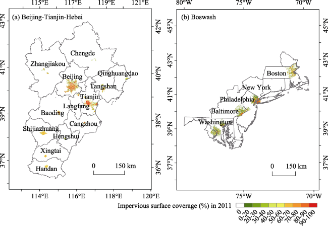
Figure 1 Overview of the study area |
Table 1 Landscape metrics and its ecological meaning |
| Landscape metric | Calculated formula | Ecological meaning |
|---|---|---|
| PLAND | ${{P}_{i}}=\frac{\sum\limits_{j=1}^{m}{{{a}_{ij}}}}{A}\text{*}100%$① | The area proportion of a certain type landscape to the total landscape area |
| Landscape shape index | $LSI=\frac{0.25E}{\sqrt{A}}$② | The measure of patches aggregation or discrete, the higher value LSI is, the more discrete the patches are |
(1) where i=1, 2, 3…, n represents the types of patches; j=1, 2, 3…, m represents the number of patches; aij represents the area of type i, and patch j; A represents the total area of patches. (2) where LSI represents the value of landscape shape index; E represents total patches perimeter; A represents the total patches area. |
Table 2 Descriptions of ecological-living-production land |
| 1st Level Class | Subclass | Description |
|---|---|---|
| Ecology land | Forestland | Such regions include woodlands, shrub lands, forest lands, etc. |
| Grassland | Such regions include high coverage grasslands, medium coverage grasslands, and low coverage grasslands | |
| Water body | Such regions include river canals, lakes, reservoir ponds, beaches, etc. | |
| Production land | Agricultural production land | Such regions include paddy lands and arid lands |
| Industrial production land | Such regions include factories, quarries, mining, and oil-field wastes outside cities as well as land for special uses, such as roads and airports | |
| Living land | Urban living land | Such regions include built-up areas of large, medium and small cities and counties |
| Rural living land | Such regions include rural settlements outside cities and counties | |
| Others | Unused land | Unused land such as sandy land, gobi, etc. |
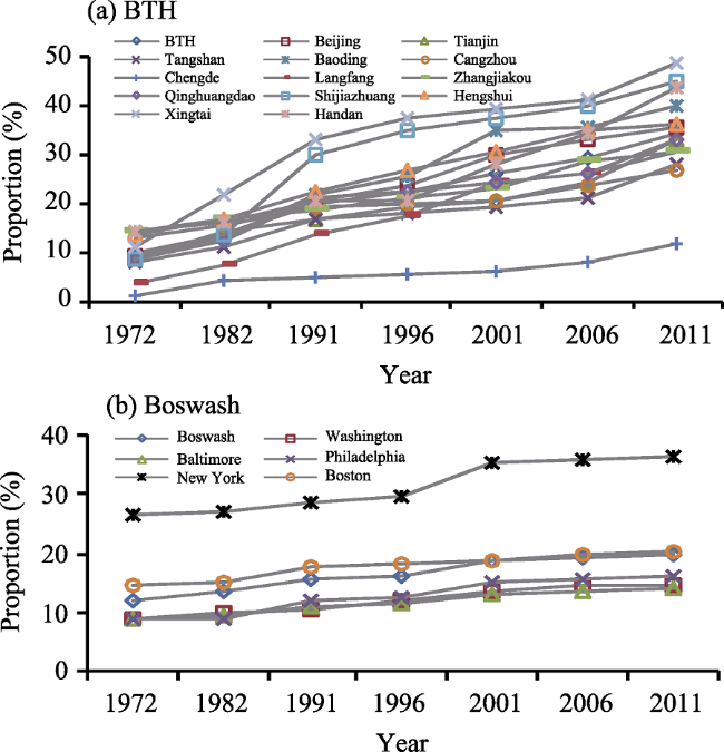
Figure 2 Proportions of the impervious surface in the BTH and Boswash, respectively, from 1972 to 2011 |
Table 3 Growth rates of the impervious surface in the BTH and Boswash |
| 1972-1982 | 1982-1991 | 1991-2001 | 2001-2011 | 1972-2011 | ||||||
|---|---|---|---|---|---|---|---|---|---|---|
| Overall variation (km2) | Variation rate (km2 yr-1) | Overall variation (km2) | Variation rate (km2yr-1) | Overall variation (km2) | Variation rate (km2yr-1) | Overall variation (km2) | Variation rate (km2yr-1) | Overall variation (km2) | Variation rate (km2yr-1) | |
| BTH | 262.60 | 26.26 | 482.12 | 53.57 | 477.99 | 47.80 | 635.13 | 63.51 | 1857.84 | 47.63 |
| Boswash | 256.34 | 25.63 | 403.02 | 44.78 | 498.34 | 49.83 | 127.73 | 12.73 | 1285.43 | 32.96 |
| Beijing | 135.36 | 13.53 | 194.70 | 21.63 | 288.89 | 28.89 | 160.96 | 16.10 | 779.91 | 19.99 |
| Tianjin | 113.84 | 11.38 | 63.11 | 7.01 | 76.16 | 7.61 | 274.89 | 27.49 | 528.00 | 13.54 |
| Tangshan | 16.99 | 1.70 | 34.35 | 3.82 | 34.35 | 3.44 | 49.53 | 4.95 | 113.60 | 2.91 |
| Baoding | 11.25 | 1.13 | 22.81 | 2.53 | 33.56 | 3.36 | 13.86 | 1.39 | 81.48 | 2.09 |
| Cangzhou | 3.29 | 0.32 | 5.71 | 0.63 | 2.03 | 0.20 | 9.19 | 0.90 | 20.22 | 0.52 |
| Chengde | 2.90 | 0.29 | 0.65 | 0.06 | 1.11 | 0.11 | 5.56 | 0.56 | 10.22 | 0.26 |
| Langfang | 7.20 | 0.72 | 10.66 | 1.18 | 18.21 | 1.82 | 11.01 | 1.10 | 47.08 | 1.21 |
| Zhangjiakou | 3.88 | 0.39 | 3.46 | 0.38 | 7.48 | 0.75 | 11.92 | 1.19 | 26.74 | 0.69 |
| Qinhuangdao | 5.64 | 0.56 | 12.31 | 1.36 | 4.23 | 0.42 | 12.86 | 1.28 | 35.04 | 0.89 |
| Shijiazhuang | 25.27 | 2.53 | 77.10 | 8.57 | 35.18 | 3.51 | 34.69 | 3.47 | 172.24 | 4.42 |
| Hengshui | 1.59 | 0.16 | 3.63 | 0.40 | 5.22 | 0.52 | 3.36 | 0.34 | 13.80 | 0.35 |
| Xingtai | 12.66 | 1.26 | 13.18 | 1.46 | 8.04 | 0.80 | 11.43 | 1.14 | 45.31 | 1.16 |
| Handan | 3.15 | 0.32 | 9.39 | 1.04 | 17.68 | 1.77 | 34.30 | 3.43 | 64.52 | 1.65 |
| New York | 14.76 | 1.48 | 40.54 | 4.50 | 171.74 | 17.17 | 29.68 | 2.97 | 256.72 | 6.58 |
| Washington | 39.92 | 3.92 | 38.61 | 4.29 | 116.73 | 11.67 | 42.69 | 4.27 | 237.95 | 6.10 |
| Baltimore | 11.07 | 1.10 | 23.77 | 2.64 | 39.83 | 3.98 | 11.40 | 1.14 | 86.07 | 2.20 |
| Philadelphia | 12.28 | 1.23 | 125.62 | 12.56 | 125.40 | 12.54 | 50.76 | 5.07 | 314.06 | 8.05 |
| Boston | 13.06 | 1.30 | 135.24 | 13.52 | 47.23 | 4.72 | 72.93 | 7.29 | 268.46 | 6.88 |
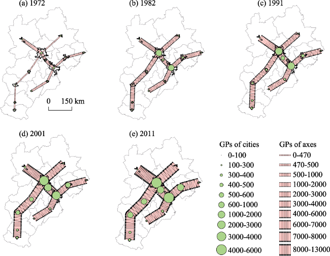
Figure 3 Spatial patterns of the gravity in the BTH (GPs represents gravitational potentials) |
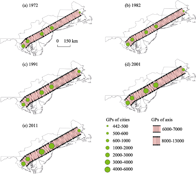
Figure 4 Spatial patterns of the gravity in the Boswash (GPs represents gravitational potentials) |
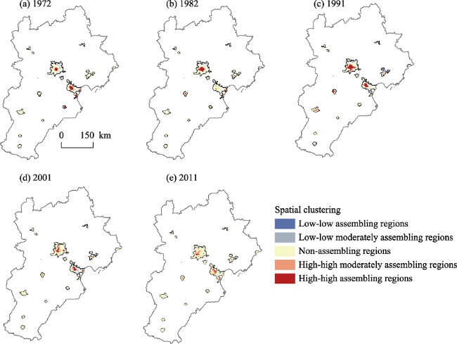
Figure 5 Spatial hotpot map of impervious surface in the BTH at urban-agglomeration scale |
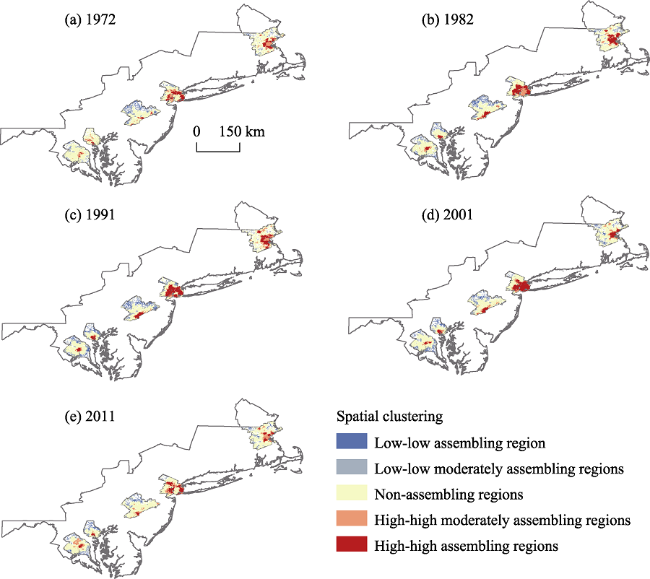
Figure 6 Spatial hotpot map of the impervious surface in the Boswash at urban agglomeration scale |
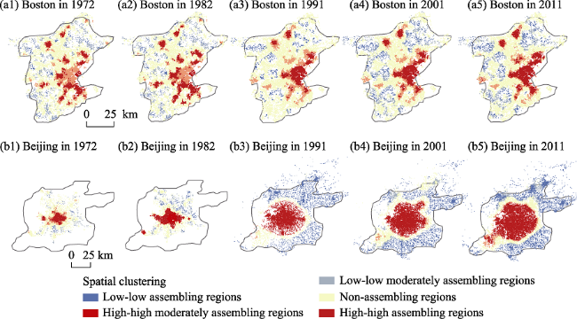
Figure 7 Spatial hotpot map of impervious surface at urban scale |
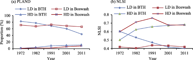
Figure 8 Landscape metrics of the BTH and Boswash (LD represents low-density impervious surfaces, and HD represents high-density impervious surfaces) |
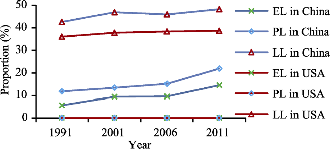
Figure 9 Ecological-living-production land area proportions of the BTH and Boswash |
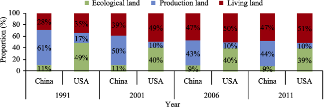
Figure 10 Proportions of the impervious surface of ecological, living, and production land (note: EL, PL, and LL represent ecological, living, production land, respectively) |
The authors have declared that no competing interests exist.
| [1] |
|
| [2] |
|
| [3] |
|
| [4] |
|
| [5] |
|
| [6] |
|
| [7] |
|
| [8] |
|
| [9] |
|
| [10] |
|
| [11] |
|
| [12] |
|
| [13] |
|
| [14] |
|
| [15] |
|
| [16] |
|
| [17] |
|
| [18] |
|
| [19] |
|
| [20] |
|
| [21] |
|
| [22] |
|
| [23] |
|
| [24] |
|
| [25] |
|
| [26] |
|
| [27] |
|
| [28] |
|
| [29] |
|
| [30] |
|
| [31] |
|
| [32] |
|
/
| 〈 |
|
〉 |