Research Articles

A GIS-based modeling of snow accumulation and melt processes in the Votkinsk reservoir basin

  • Sergey V. PYANKOV 1 ,
  • Andrey N. SHIKHOV , 1 ,
  • Nikolay A. KALININ 2 ,
  • Eugene M. SVIYAZOV 2
Expand
  • 1. Department of Cartography and Geoinformatics, Perm State University, 15 Bukireva Street, 614990 Perm, Russia
  • 2. Department of Meteorology and Atmosphere Protection, Perm State University, 15 Bukireva Street, 614990 Perm, Russia

Author: Andrey N. Shikhov, Associate Professor, E-mail:

Received date: 2016-10-11

  Accepted date: 2017-02-24

  Online published: 2018-02-10

Supported by

RFBR project 14-05-00317-a

Copyright

Journal of Geographical Sciences, All Rights Reserved

Abstract

Coupled hydrological and atmospheric modeling is an efficient method for snowmelt runoff forecast in large basins. We use short-range precipitation forecasts of mesoscale atmospheric Weather Research and Forecasting (WRF) model combining them with ground-based and satellite observations for modeling snow accumulation and snowmelt processes in the Votkinsk reservoir basin (184,319 km2). The method is tested during three winter seasons (2012-2015). The MODIS-based vegetation map and leaf area index data are used to calculate the snowmelt intensity and snow evaporation in the studied basin. The GIS-based snow accumulation and snowmelt modeling provides a reliable and highly detailed spatial distribution for snow water equivalent (SWE) and snow-covered areas (SCA). The modelling results are validated by comparing actual and estimated SWE and SCA data. The actual SCA results are derived from MODIS satellite data. The algorithm for assessing the SCA by MODIS data (ATBD-MOD 10) has been adapted to a forest zone. In general, the proposed method provides satisfactory results for maximum SWE calculations. The calculation accuracy is slightly degraded during snowmelt periods. The SCA data is simulated with a higher reliability than the SWE data. The differences between the simulated and actual SWE may be explained by the overestimation of the WRF-simulated total precipitation and the unrepresentativeness of the SWE measurements (snow survey).

Cite this article

Sergey V. PYANKOV , Andrey N. SHIKHOV , Nikolay A. KALININ , Eugene M. SVIYAZOV . A GIS-based modeling of snow accumulation and melt processes in the Votkinsk reservoir basin[J]. Journal of Geographical Sciences, 2018 , 28(2) : 221 -237 . DOI: 10.1007/s11442-018-1469-x

1 Introduction

A river’s hydrological regime in a cold climate zone is mainly determined by snow accumulation and snowmelt processes, because the snowmelt runoff forms 60-70% of the annual streamflow. Snowmelt floods are often observed during the spring snowmelt season and they cause considerable damage. The reliability of their forecasting is not satisfactory in some cases. To increase the forecast reliability, it is necessary to evaluate the snow water equivalent (SWE) more accurately, considering the heterogeneity of its spatial distribution. This heterogeneity is determined by the interaction between snow accumulation, snowmelt, snow sublimation and blowing processes (Kuzmin, 1961; Pomeroy et al., 1998). Therefore, the SWE calculation has a high uncertainty, especially in mountainous terrain with sparse observation networks.
Several physically-based models of snow accumulation and melt processes have been developed to calculate the SWE spatial distribution (Tarboton et al., 1996; Marks et al., 1999; Kuchment et al., 2000; Garen and Marks, 2005; Lehning et al., 2006; Quéno et al., 2016). Furthermore, statistical methods based on interpolation may be used to estimate the spatial distribution of the SWE (Carroll and Cressie, 1996; Shutov, 1998; Lopez-Moreno and Nogues-Bravo, 2006). The physically-based models of snow accumulation and melting processes are based on the solution of balance equations in grid cells. Significant volumes and low accessibility of input data, especially for large and ungauged basins, are the limitations for the use of physically-based models. Another restriction is due to the sparse and unrepresentative location of weather stations (Lehning et al., 2006). Due to these reasons, the physically-based models of snow accumulation and snowmelt processes are rarely used in large watersheds (Marks et al., 1999; Garen and Marks, 2005; Kuchment et al., 2010).
Geostatistical methods for SWE estimation are also widely applied in hydrological forecasting. For example, the U.S. National Weather Service uses the results of geostatistical simulation for assessing snow cover characteristics as the input data for a streamflow formation model (Carroll and Cressie, 1996). Given the high density of snow observation networks, an interpolation with an inverse distance weighting method and kriging or regression models are used to simulate snow depth and the SWE. The SWE assessment using regression models based on their dependence on elevation, terrain slope and solar radiation is usually considered to be the most reliable (Elder et al., 1998; Erxleben et al., 2002, Lopez-Moreno and Nogues-Bravo, 2006).
Simultaneously, the estimates of the SWE spatial distribution using ground-based observations also have limited utility over large areas. The spatial density of operational ground-based snow observations is too low to resolve small-scale variability in the SWE distribution as the distance between observations is far greater than the correlation-length scale (Bl¨oschl, 1999). This small-scale variability in the SWE distribution is due to orography and vegetation cover diversity (Bl¨oschl, 1999). The correct interpolation of SWE field measurement data is impossible in mountainous areas. Interpolation of the accumulated precipitation during the cold period provides more reliable input data for SWE estimation (Shutov, 1998).
The use of mesoscale weather forecast models significantly simplifies the SWE assessment (as well as others meteorological variables) in the cases where ground-based observations are absent (Kunstmann and Stadler, 2005; Georgakakos et al., 2014, Queno et al., 2016). The high reliability and spatial resolution of short-range precipitation forecasts in the cold season allow them to be combining with runoff formation models. The hydrological model is driven by the forecast data obtained from an atmospheric model. As a result, the lead time for runoff forecast significantly increases. Such systems of coupled atmospheric-hydrological forecasts are developed for mountain areas with high flood risk to help decision making and reduce the possible damage caused by floods (Addor et al., 2011, Verbunt et al., 2006; Zhao et al., 2009), as well as to calculate water inflow to reservoirs (Georgakakos et al., 2014).
Some snow cover characteristics (the snow-covered area, snow surface temperature and SWE) can be estimated by satellite data. However, the potential of satellite snow data is limited by a number of environmental factors (cloudiness, land cover type, terrain peculiarities and so on). Cloudiness creates a discontinuity in the spatial distribution and in time data series. Dense forest vegetation complicates snow cover identification and mapping due to snow interception and the ability to mask snow cover on the forest floor. The accuracy of satellite measurements of SWE significantly depends on the snow properties, especially the amount of liquid water (Kuchment et al., 2010).
The snow-covered area (SCA) can be estimated most reliably using remote sensing data. Its reliability is determined by Moderate Resolution Imaging Spectroradiometer (MODIS) satellite data ranging from 90% to 98% depending on the season and surface type (Hall and Riggs, 2007). Satellite-derived SCA are used for validation and calibration of the physically-based (distributed) models of snow cover (Kuchment et al., 2010)
Estimates of SWE spatial distribution can be also obtained using AMSR-E/Aqua microwave radiometer sounding data. The probable error for SWE assessment based on AMSR-E satellite data is ~25% (Chang and Rango, 2000), although it may be significantly higher for forest areas. The evaluation results of this algorithm for the European part of Russia have revealed that errors of SWE estimates can reach 200% (Nosenko et al., 2006).
Thus, the problem of SWE estimation on large watersheds with diverse environments and sparse observation networks has not been solved yet. The present work provides the results of GIS-based modelling of snow cover characteristics in a large basin. The model input is the combination of ground-based, satellite observations and mesoscale numerical weather forecast data. ESRI ArcGis 10.1 software is used for the calculations. The presented technique was applied to the area including the Votkinsk Reservoir catchment (S = 184319 km2). The studied basin is characterised by diverse natural conditions and the sparse location of ground-based weather stations (Figure 1). The simulation period includes the 2012-2015 winter seasons.
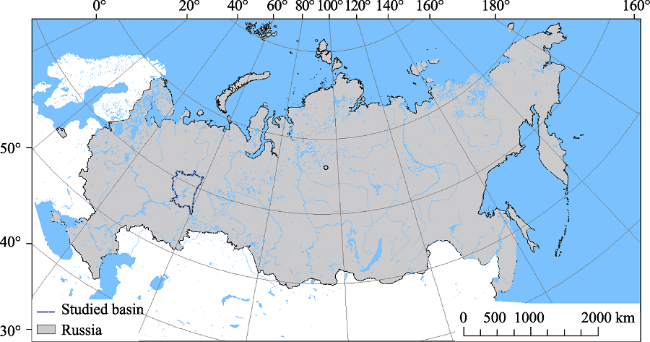
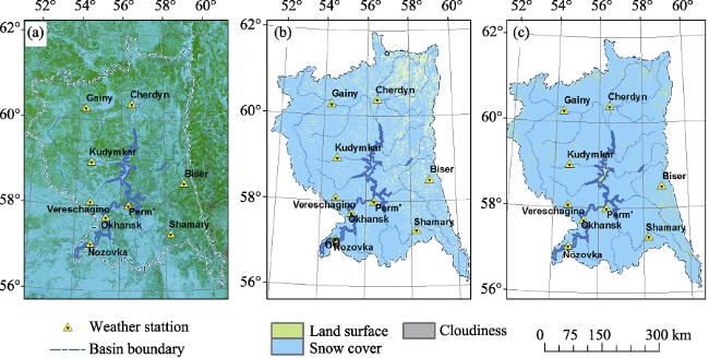
Figure 1 The geographical location of the Votkinsk reservoir basin in Russia

2 Study area

The Votkinsk Reservoir basin is located in the north-eastern part of the Volga river basin, and has an area of 184319 km2 (Figure 1). The minimum elevation within the studied basin is 89 m, and the maximum elevation is 1519 m. The western and central parts of the studied basin belong to the East-European plain with the altitude from 88 m up to 446 m in height. The eastern part of the studied basin is located in the Ural Mountain system and is subdivided into the Northern and Middle Ural. The typical point elevation for the Middle Ural is 400-900 m in height and it increases up to 800-1519 m in height for the Northern Ural. Approximately 70% of the studied area is covered by forests. The recovered mixed spruce-birch forest prevails in most of the watershed. The undisturbed dark coniferous forests cover significant areas north of 60°N, and the recovered small-leaved forests prevail in the southern part of the basin (Figure 2).
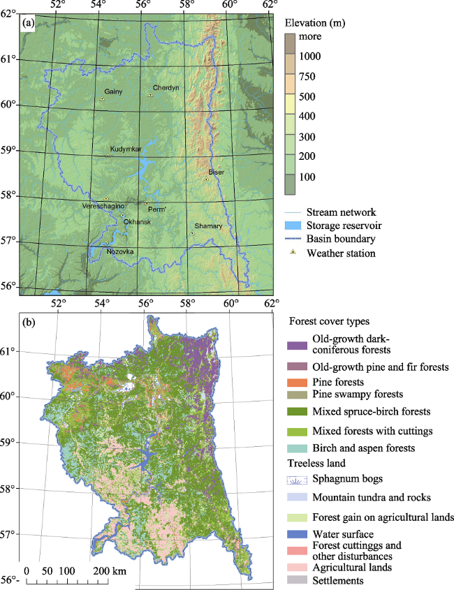
Figure 2 Topography (a) and vegetation types (b) of the Votkinsk reservoir basin, Russia
The climate of the studied catchment is temperate-continental and characterised by long and cold winters. Annual precipitation ranges from 500 mm in the southwest part of the basin to 900-1100 mm in the mountainous north-eastern areas. During the cold season (from November to March), the total precipitation ranges from 150-200 mm in the flat part of the basin up to 300-350 mm in the mountains. Snow cover usually forms in the middle of October in the mountainous areas, and in early November in the flat part of the basin. It melts in the middle of April for the plain part and at the beginning of May for the mountainous part. The maximum snow depth and SWE forms in the end of March. It ranges usually ranges from 50-60 cm in the southwestern part of the basin to 120 cm in the mountainous north-eastern areas. The maximum SWE ranges from 130-180 mm at the plain part of the watershed and 200-250 mm at the uplands to ~300 mm and even higher in the northeastern areas.

3 Data collection and methods

3.1 Data sources

The methodology of SWE assessment is based on the summing of cold period precipitation, considering their phases, snowmelt during thaws, snow interception and sublimation from the snow surface. Spring snowmelt intensity is assessed according to the method of Kuzmin, which is based on the snow cover heat balance equation when the melting snow surface temperature is 0°С (Kuzmin, 1961). The snow cover characteristics are calculated with a 24 h time step and 3000 m spatial resolution. Calculations with a higher grid step are not appropriate. The input data used for modelling is as follows:
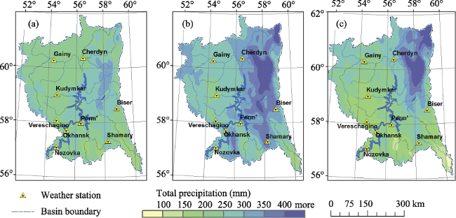
Forecast fields of solid and liquid precipitations, wind speed at 10 m height, temperature and air humidity at 850 hPa isobaric surface, computed by the mesoscale weather forecast model WRF with 10 km grid step;
Observations data from 34 ground-based weather stations located both at the studied watershed and outside it (air temperature and humidity, total and lower cloudiness, daily total precipitations);
Underlying surface data: the digital elevation model of the watershed based on the GMTED2010 elevation matrix (Figure 2a) and an actual land cover map based on Terra/ Aqua MODIS satellite images (Figure 2b);
SWE field measurement (snow survey) data from the weather stations, to validate the SWE simulation results, and MODIS-estimated snow-covered area during spring snowmelt seasons.
Forecast snow and rain precipitations fields computed by the mesoscale Weather Research and Forecasting (WRF) atmospheric model v3.3 have been used as input data for the SWE assessment. The detailed description of the WRF model is presented in (Skamarock et al., 2008). The WRF model is widely used both for research projects and operational forecast services, as well as for high resolution meteorological forecasts in flood warning systems (Kumar et al., 2008; Zhao et al., 2009).
The WRF model has been run at the computing cluster of Perm State University. The calculations have been done using the ARW dynamical core for the 48-hour period starting at 00 UTC. The model is run with 10 km grid step and 60 second time step. Output data is provided every 3 hours. The global GFS/NCEP model data are the initial conditions for the WRF model run. The grid size of WRF model was 2000 km × 2000 km. The output data for the period of 15-39 hours from the forecast start were used for further SWE calculations, to provide matching with the timing of precipitation measurements at the weather stations. The results of the cold period (from November to March) total precipitations calculation based on the WRF model are presented at Figure 3.
Figure 3 Total precipitation for 2012/13 (a), 2013/14 (b), and 2014/15 (c) cold seasons, calculated by WRF model

3.2 Main methods

3.2.1 Processing of meteorological data
Ground-based observations data from 34 weather stations located both at the studied watershed and outside it (air temperature and humidity, total and lower cloudiness, daily total precipitations) have been used as input data for snow accumulation and melt model. Simulation of spatial distribution of meteorological variables has been done using interpolation methods with an altitude-dependent-regression. Similar methods for data processing in distributed hydrological models are described by Motoya et al. (2001) and Klok et al. (2002).
Air temperature and humidity interpolation have been based on weather stations observations, using the interpolation method with altitude-dependent-regression. Altitude gradients have been calculated by the WRF model data on temperature and air humidity at the 850 hPa isobaric height per each observation period as well as using digital elevation model.
Wind speed distribution is computed from the WRF model data. To consider the wind speed decrease in a forest, the reducing factors recommended by Koren’ (1991) have been introduced. These factors are equal to 0.15 for dark coniferous forests; 0.2 for mixed forests and 0.25 for small-leaved forests.
Daily upward solar radiation during snowmelt season is calculated according to DEM and water vapour pressure data using the algorithm implemented in the System for Automatized Geoscientific Analysis (SAGA) software. This algorithm is described in detail by Wilson and Gallant (2000). The influence of total and lower cloudiness, and forest vegetation have been considered with the reducing factors suggested by Kuzmin (1961), and also adapted by Kuchment et al. (2010) for spatially distributed snowpack model. The total and lower cloudiness has been interpolated according to ground-based weather stations. Different reducing factors have also been used to assess total upward solar radiation in different forests types, when the average forest projective cover is 0.7 (Kuzmin, 1961).
The calculation of snow cover albedo has a high uncertainty because the albedo depends on snow surface age, snow depth, snow-covered area, cloudiness and other factors. Freshly fallen snow albedo is 90% but at the end of a snowmelt period it reduces to 50% and lower. Besides, the snow albedo in a forest is significantly (at 0.1‒0.15) lower than in a treeless area (Melloh et al., 2001). In different snowpack models, the albedo is calculated with empiric dependencies from snow surface age (Wigmosta et al., 1994; Motoya et al., 2001), according to the data about snow cover density changes (Kuchment et al., 2010), or using satellite data. The implementation of physically-based models for albedo calculations, for example (Melloh et al., 2001) for large basins is rather complicated. The approach for albedo calculation considering the main factors influencing its changes proposed by Gordeev (2013) has been modified in the present research. The results of calculation of spatial distribution of snow cover albedo according to the present methodology are presented at Figure 4.
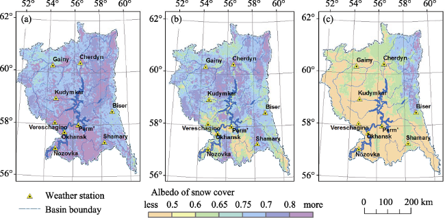
Figure 4 Snow cover albedo dynamics during snowmelt season: a) 03/15/2015; b) 04/15/2015; c) 05/05/2015
3.2.2 Calculation of snow sublimation in snow accumulation season
The snowpack losses include snowmelt and snow sublimation. Snowmelt intensity during autumn and winter thaws is calculated with temperature-index method. The degree-day factor has been calculated using calibration considering the land cover type. The influence of solar radiation is minimal during this period, therefore it has not been considered during the calculations.
Snow cover sublimation includes evaporation from the snow surface with intensity depending on air humidity and wind speed, and sublimation of intercepted snow. The calculation of total snow cover sublimation during cold period is done with the technique described in Karpechko and Bondarik (2010):
Esum=Ei+E (1)
where Ei is the sublimation of intercepted snow, E is the sublimation from the snow surface
${{E}_{i}}=k\cdot d\cdot LAI\cdot n$ (2)
where LAI is leaf area index, d denotes an average deficit of saturation air vapour pressure, n signifies the amount of days, k is the empiric reducing factor (accepted to be 0,03)
$E=(0.24+0.05\cdot {{U}_{10}})\cdot D\cdot n$ (3)
where U10 is wind speed at 10 m altitude.
The leaf area index LAI depends on forest vegetation density and forest type. LAI was used to calculate intensity of snow interception for several snow cover models (Pomeroy et al., 1998; Gelfan et al., 2004; Kuchment et al., 2010). LAI has been obtained by MODIS product MOD15A2 (8-day LAI and FPAR). The more detailed description of this product is presented by Myneni et al. (2002). The MODIS data for March, 2015 is used because there was no cloudiness above the studied area at that time.
The total snow evaporation during a cold period estimated according to the above mentioned technique ranges from 10-15 mm in small-leaved forests to 50 mm in dark coniferous and pine forests (Figure 5). These values are consistent with field measurements data in neighbouring region (Shutov, 1998). The maximum snow evaporation rate is observed in March because of the low relative air humidity.
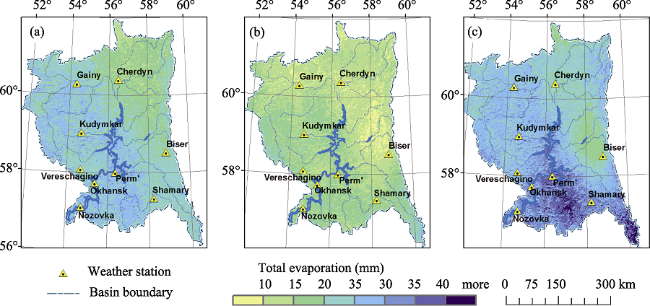
Figure 5 Total snow evaporation in 2012/13 (a), 2013/14 (b) and 2014/15 (c) cold seasons
3.2.3 Calculation of maximum snow water equivalent
The maximum SWE is formed at the plain part of the studied area in March and at the mountainous part at the beginning of April. The periods of stable and unstable snow accumulation are observed in the studied basin. Thaws occur infrequently during stable snow accumulation period, from December to February. In this period, the snowpack losses are formed mainly due to snow sublimation processes. In the autumn period, thaws are regularly observed. Consequently, snow cover repeatedly appears and disappears at the flat part of the basin, but the steady SWE increase is observed in Ural mountains. The results of the maximum SWE estimation at the studied watershed are shown in Figure 6.
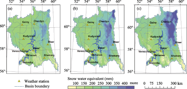
Figure 6 Maximum snow water equivalent during 2012/13 (a), 2013/14 (b) and 2014/15 (c) cold seasons
The spatial distribution of SWE is characterised by substantial spatial heterogeneity and interannual variability, induced by atmospheric circulation peculiarities of each winter season. For example, an intensive zonal atmospheric process was observed in the 2014/15 cold period. Large amount of precipitation fell at the meridional oriented mountain ridges of Northern Ural as a result of the barrier effect. The maximum SWE on the western slopes of the Urals increased to 500 mm or more. On the contrary, meridional circulation prevailed in the 2012/13 cold period. Therefore, the barrier effect was insignificant and the spatial distribution of precipitation was relatively homogeneous. Zonal atmospheric processes were prevailed also in November and December of 2013, but the meridional circulation was typical for January-February 2014. Thus, the precipitation amounts and snow accumulation rate at these periods differ significantly. In general, the largest SWE was formed on the mountainous part of the watershed in 2015, and on the plain part it was formed in 2014.
3.2.4 Spring snowmelt modeling
Simulation of spatial distribution of snowmelt intensity has been implemented by GIS technology, using modified heat balance method, proposed by PP Kuzmin (Kuzmin, 1961). This method allows us to calculate the components of snow cover energy balance based on standard meteorological observations data and simulated incoming solar radiation (including cloudiness influence).
The heat balance equation, neglecting its minor components, is written as follows:
$W={{W}_{R}}+{{W}_{A}}+{{W}_{E}}$ (4)
where WR denotes radiation balance, WA denotes sensible turbulent heat flux, and WE represents latent heat flux for snow sublimation and from water vapor condensation on the snow surface.
The radiation component of snowmelt rate (MR) is calculated by:
${{M}_{R}}+{{Q}_{sw}}-{{Q}_{ls}}+{{Q}_{lw}}$ (5)
where Qsw is the short-wave radiation balance, Qls denotes upward longwave radiation from snow and Qlw is downward long wave radiation. The radiation balance components are calculated as follows (6‒8):
${{Q}_{sw}}=0.125(Q+q)(1-R)(1-0.2{{N}_{total}}-0.47{{N}_{lower}})$ (6)
${{Q}_{ls}}=\varepsilon \sigma T_{0}^{4}$ (7)
${{Q}_{lw}}=(\varepsilon \sigma T_{0}^{4})(0.62+0.05{{e}^{0.5}}(1+0.12{{N}_{total}}+0.12{{N}_{lower}})$ (8)
where Q+q represents the short-wave direct and diffuse radiation flux (under clear sky conditions) for the day, R denotes albedo of snow cover, ${{N}_{total}}$ and ${{N}_{lower}}$ are the percentage of total cloudiness and lower level cloudiness respectively, T0 represents air absolute temperature, e denotes water vapor pressure at a 2 m height, σ is the Stefan-Boltzmann constant, and ε signifies the effective emissivity of the snowpack taken equal to 0.99 in this study.
The advective component of snowmelt is determined by the turbulent heat exchange between snow cover and atmosphere, and latent heat flux from condensation of water vapor on the snow surface:
${{M}_{A}}=k(1+0.544{{U}_{10}})({{T}_{2}}-{{T}_{0}}+1.75({{e}_{2}}-{{e}_{0}}))$ (9)
where U10 represents wind speed at 10 m height, T2 and e2 denotes air temperature and water vapor pressure at 2 m height, T0 is the snow surface temperature, e0 is the saturated water vapour pressure at the snow surface temperature. The factor k before formula (9) depends on the model time step; it is assumed to be 0.434 in the case of calculations with 12-hours steps.
Evaporation (E) from snow cover is calculated by the Kuzmin method (Kuzmin, 1961)
$E=0.18+0.098{{U}_{10}}({{e}_{2}}-{{e}_{0}})$ (10)
Application of energy balance method for simulation of snowmel.t requires extensive data processing, which is not always acceptable in operational forecasting. Thereby, we also use a simple temperature-index model for snowmelt simulation. In simple model, the snowmelt intensity is calculated from the average daily temperature taking into account land cover/land use type. We made a comparison of the simulation results for these two models. The output data of both model versions is snow covered area, snow water equivalent and meltwater outflow to the catchment. The results of SWE dynamics simulation during the spring snowmelt period in 2015 are shown in Figure 7.
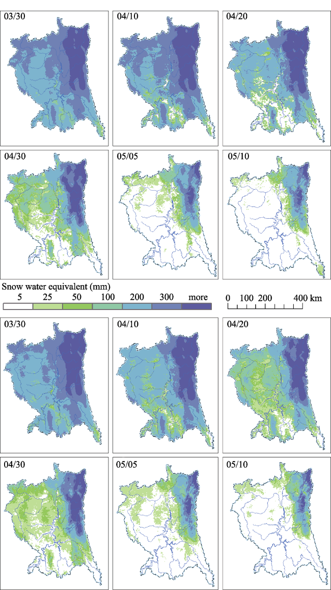
Figure 7 The simulated spatial distribution of SWE in 2014/15 snowmelt season by Kuzmin method (top line) and by temperature-index method (bottom line)

4 Results and discussion

4.1 Estimation of accuracy of simulated precipitation by the WRF-ARW model

The reliability of calculation of precipitation amounts in cold period was estimated by comparing the actual and simulated monthly total precipitation at 34 weather stations. The results are presented in Table 1. The following criteria were used to accuracy assessment;
Table 1 Estimation of accuracy of simulated precipitation in cold seasons by the WRF-ARW model
Parameters Year Month
November December January February March
Xm 2012/13 61.8 29.5 33.8 15.1 50.5
2013/14 65.0 59.5 39.6 34.7 44.9
2014/15 24.1 45.1 42.3 28.6 17.0
Xs 2012/13 65.0 32.6 33.9 21.9 66.6
2013/14 64.7 62.5 44.0 32.2 67.2
2014/15 28.0 54.0 49.2 43.0 27.8
$\Delta \overline{X}$ 2012/13 10.0 4.9 5.2 7.7 17.8
2013/14 12.0 9.3 7.2 6.2 24.1
2014/15 5.8 9.3 9.5 15.0 11.1
RMSE 2012/13 12.1 6.9 6.2 8,6 21.1
2013/14 15.4 11.6 9.1 8.7 27.0
2014/15 6.6 11.1 12.0 16.1 12.5
RMSE/Xm,% 2012/13 20.0 23.0 18.0 57 42.0
2013/14 23.0 20.0 23.0 25 60.0
2014/15 27.0 25.0 28.0 56 73.0
2014/15 6.1 10.7 10.8 16.1 11.2
The mean absolute forecast error
$\Delta \overline{X}=\sum{({{X}_{m}}-{{X}_{s}})}/n$, (11)
where $\Delta \overline{X}$ is a mean absolute error of precipitation forecast for the month, n denotes the number of weather stations used in comparison (in this case n = 34), Xm signifies monthly total precipitation according to the weather station and Xs denotes monthly total precipitation according to WRF model data.
Root mean square error of forecast (RMSE)
$RMSE=\sqrt[{}]{\frac{1}{n}\sum\limits_{i=1}^{n}{{{({{X}_{m}}-{{X}_{s}})}^{2}}}}$ (12)
Comparison of ground-based observations and WRF model forecasts has revealed that the model overestimates the precipitation amount in most cases. Strong systematic overestimation (on average 35%-50% along the territory) has been observed in March (for the whole three years) and in February 2013, 2015. Slight overestimation (within 20%) of simulated precipitation amount is generally observed in November-January. Calculated total precipitation occurred to be 6% lower than the observed one in February 2014 (Table 1).
RMSE for the calculation of monthly total precipitation by the WRF model is within 18%‒31% (in most cases) from the average precipitation amount measured by ground-based weather stations. These results can be considered satisfactory as calculation errors value is close to measurement errors in snow precipitation at the weather stations. Solid precipitation assessment at weather stations is known to be 20%‒30% less than the actual due to the snow blowing from a precipitation gauge. RMSE increases significantly at the end of the cold period (February-March). Overestimation of simulated precipitation amounts achieves 35%‒50% on average, and to 80%‒100% at some weather stations. The model overestimates amount of large-scale and local heavy precipitation.
The largest difference between model and observed precipitation amount is typical for the weather stations located at a lower relief type, in deep river valleys in particular. At the same time, the total model precipitation exceeds the observed one less than 20% for weather stations located at highlands. The spatial resolution of forecast data explains these deviations. The WRF model with a 10 km grid step smooths the spatial distribution of precipitation without consideration of the mesoscale forms of terrain. However, the areas with maximum precipitation accumulation due to the barrier effect of meridionally oriented mountain ridges are well identified even with this grid step. The model does not reduce precipitations in river valleys, in comparison with the neighbourhood highlands if valleys width is lower than 5 km. The decrease of a grid step up to 3-5 km is able to remove this disadvantage but additional computing resources should be used to run a high resolution model for long time period.
The spatial distribution of precipitation during cold period is characterised by significant similarities. The precipitation amount increases always with the altitude, and other spatial distribution peculiarities during every winter season depend on circulation conditions. When zonal processes prevail, the barrier effect of highlands and mountains is stronger and precipitation is distributed more unevenly. Thus, according to the WRF model data more than 500 mm of precipitation fell on axis part of the Northern Ural, whereas less than 100 mm of precipitation observed to the east of the mountain ridge. When the zonal circulation was reduced (for example, in 2012-2013 winter season), the barrier effect of mountains is smoothed and precipitation is distributed more evenly.

4.2 Accuracy assessment of snow water equivalent simulation

The model SWE at the Votkinsk reservoir basin is validated against the SWE field measurements data along the forest and clearing routes of 24 weather stations. To compare with the snow survey data, the simulated SWE was extracted from the model grid cell. The spatial distribution of these cells corresponds to the snow surveys routes of weather stations. Reliability of SWE estimation has been checked by both the method suggested by Kuzmin and by temperature-index method. The average SWE according to forest and clearing snow survey routes and its RMSE calculation are presented in Figure 8, whereas Figure 9 presents the comparison of measured and simulated SWE at individual weather stations.
Figure 8 Accuracy assessment of simulated SWE seasonal dynamics: a) - 2012/13, treeless areas; b) - 2012/13, forest; c) - 2013/14, treeless areas; d) - 2013/14, forest; e) - 2014/15, treeless areas; d) - 2014/15, forest
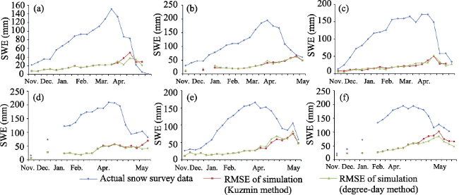
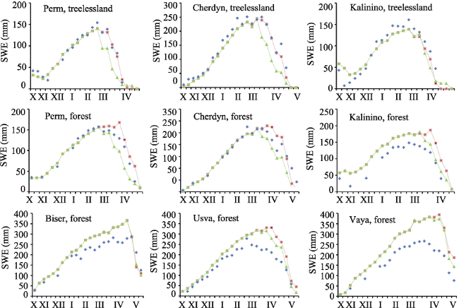
Figure 9 Seasonal dynamics of measured (blue points), simulated using Kuzmin method (red line) and simulated using degree-day method (green line) SWE (in mm) at selected stations within the study area for the season from October 2014 to May 2015
The increase of the absolute calculation error should be mentioned during the snow accumulation period. However, RMSE did not exceed 25% from the observed SWE (except one case in 2015) during the maximum snow accumulation period (in March). This RMSE value may be considered satisfactory since the snow survey data are not considered to be representative (particularly in the mountainous part of the catchment). RMSE of snow water equivalent estimation increases significantly during the spring snowmelt since local factors of snow redistribution begin to effect.
When calculating the spring snowmelt by Kuzmin method there is an underestimation of snowmelt intensity in forests but it is overestimated in open terrain. On the contrary, we observed the overestimation of snowmelt intensity in forests when using the temperature-index method. In general, the results of both calculation methods are comparable.
The difference of observed and measured SWE at the studied basin is systematic in some cases. For example, the systematic overestimation of SWE was observed in February-March
2015 that was caused by the total precipitation overestimation by the WRF model at that period. The greatest divergence between the measured and simulated SWE are typical for the mountainous areas (Figure 9). Snow survey data in the mountainous part of the Urals obtained in deep river valleys are not representative for the neighbouring territory.

4.3 Accuracy estimation of snow-covered area simulation during snowmelt period

The representativeness and reliability of SWE measurements decrease and their frequency becomes insufficient during spring snowmelt period. Therefore, the satellite data about a snow-covered area (SCA) become necessary for operational monitoring of snowmelt. The main source of SCA satellite measurements is the Earth Observing System MODIS radiometer. The algorithm of snow cover mapping by MODIS data (ATBD-MOD10) is based on a Normalized Differential Snow Index NDSI (Hall et al., 2001). ATBD-MOD10 algorithm has been tested by authors while comparing a huge amount of MODIS images with LANDSAT satellite data. The threshold value of NDSI for identifying snow covered area (SCA) is recommended to be 0.4. According to the algorithm developers, the accuracy of SCA estimation ranges from 90% to 98% in dependence on a season and vegetation type (Hall and Riggs, 2007).
Dense forest vegetation complicates snow cover identified by ATBD-MOD10 algorithm. Snow cover reliably identified only for deciduous forests. To estimate the SCA in the mixed and coniferous forests, it needs to use other NDSI threshold values. Regional NDSI threshold values have been calculated while comparing MODIS and LANDSAT satellite images. The threshold regional value for woodless areas is set to 0.35; and for forest areas it is 0.1. The MCD12Q1 (Land Cover Type) data was used to create forest mask of studied basin.
The comparison of the SCA maps created using standard and modified algorithms is presented in Figure 10. Satellite data have been received on April 3, 2015 when the entire watershed was covered by snow. The SCA estimated using the modified algorithm was about 96%, but it decreased to 78% according to the ATBD-MOD10 data. Thus, the change of the threshold values recommended in ATBD-MOD10 increase the accuracy of SCA estimation by MODIS satellite data.
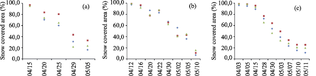
Figure 10 Assessment of snow-covered area by MODIS data of April 3, 2015: a) RGB bands 7-2-1; b) Snow-covered area calculated by ATBD-MOD10; c) Snow-covered area calculated by modified algorithm
The SCA estimated by the modified algorithm was compared to the simulated SCA (Figure 11). The difference between the actual and estimated SCA does not exceed 10% in most cases. The SCA estimated using Kuzmin method turned to be slightly overestimated in 2013 and 2015, whereas the SCA calculated by temperature-index method often turns to be underestimated. In general, it is difficult to determine a method providing more accurate results.
Figure 11 MODIS-observed (blue symbol), simulated by the Kuzmin method (red symbol) and simulated by degree-day method (green symbol) snow-covered area for the 2013 (a), 2014 (b) and 2015 (c) snowmelt seasons

5 Conclusion

The combination of ground-based observations, satellite data and mesoscale numerical weather forecast models is a promising approach to estimate SWE spatial distribution at large watersheds with mountainous areas and sparse observation networks. The results of these studies show the relevance and reliability of the presented method application for the Votkinsk Reservoir basin and the advantages of its further development at neighbouring or similar regions. The forecast precipitation fields by the WRF model have been used to estimate the spatial distribution of the SWE. The significant errors revealed while comparing field measurements data to model results are caused by local features of snow survey route locations.
The use of the digital elevation model and MODIS data (vegetation cover maps and leaf area index) allows to simulate SWE spatial distribution with high resolution considering the influence of landscape conditions of snow accumulation processes. The suggested methodology realised on a GIS-technology basis provides users with visual results.
The algorithm for snow cover identification by MODIS data (ATBD-MOD10) has been modified to be used for forest areas. It allows us to decrease errors when estimating the SCA by satellite data and to use MODIS data for the model validation more efficiently.

The authors have declared that no competing interests exist.

[1]
Addor N, Jaun S, Fundel Fet al., 2011. An operational hydrological ensemble prediction system for the city of Zurich (Switzerland): Skill, case studies and scenarios.Hydrology and Earth System Sciences, 15: 2327-2347.The Sihl River flows through Zurich, Switzerland's most populated city, for which it represents the largest flood threat. To anticipate extreme discharge events and provide decision support in case of flood risk, a hydrometeorological ensemble prediction system (HEPS) was launched operationally in 2008. This model chain relies on limited-area atmospheric forecasts provided by the deterministic model COSMO-7 and the probabilistic model COSMO-LEPS. These atmospheric forecasts are used to force a semi-distributed hydrological model (PREVAH), coupled to a hydraulic model (FLORIS). The resulting hydrological forecasts are eventually communicated to the stakeholders involved in the Sihl discharge management. This fully operational setting provides a real framework with which to compare the potential of deterministic and probabilistic discharge forecasts for flood mitigation. To study the suitability of HEPS for small-scale basins and to quantify the added-value conveyed by the probability information, a reforecast was made for the period June 2007 to December 2009 for the Sihl catchment (336 km). Several metrics support the conclusion that the performance gain can be of up to 2 days lead time for the catchment considered. Brier skill scores show that overall COSMO-LEPS-based hydrological forecasts outperforms their COSMO-7-based counterparts for all the lead times and event intensities considered. The small size of the Sihl catchment does not prevent skillful discharge forecasts, but makes them particularly dependent on correct precipitation forecasts, as shown by comparisons with a reference run driven by observed meteorological parameters. Our evaluation stresses that the capacity of the model to provide confident and reliable mid-term probability forecasts for high discharges is limited. The two most intense events of the study period are investigated utilising a novel graphical representation of probability forecasts, and are used to generate high discharge scenarios. They highlight challenges for making decisions on the basis of hydrological predictions, and indicate the need for a tool to be used in addition to forecasts to compare the different mitigation actions possible in the Sihl catchment. No definitive conclusion on the model chain capacity to forecast flooding events endangering the city of Zurich could be drawn because of the under-sampling of extreme events. Further research on the form of the reforecasts needed to infer on floods associated to return periods of several decades, centuries, is encouraged.

DOI

[2]
Bl¨oschl G, 1999. Scaling issues in snow hydrology.Hydrological Processes, 13: 2149-2175.

DOI

[3]
Carroll S S, Cressie N, 1996. A comparison of geostatistical methodologies used to estimate snow water equivalent.Water Resources Bulletin, 32: 267-278.ABSTRACT: The need to monitor and forecast water resources accurately, particularly in the western United States, is becoming increasingly critical as the demand for water continues to escalate. Consequently, the National Weather Service (NWS) has developed a geostatistical model that is used to obtain areal estimates of snow water equivalent (the thtal water content in all phases of the snowpack), a major source of water in the West. The areal snow water equivalent estimates are used to update the hydrologic simulation models maintained by the NWS and designed to produce extended streamflow forecasts for river systems throughout the United States. An alternative geostatistical technique has been proposed to estimate snow water equivalent. In this research, we describe the two methodologies and compare the accuracy of the estimates produced by each technique. We illustrate their application and compare their estimation accuracy using snow data collected in the North Fork Clearwater River basin in Idaho.

DOI

[4]
Chang A T C, Rango A, 2000. Algorithm Theoretical Basis Document for the AMSR-E Snow Water Equivalent Algorithm, Version 3.1. Greenbelt, MD, USA, NASA Goddard Space Flight Center, 49 pp.Page 1. Cycle 18 Approved Programs Phase II First Name Last name PI InstitutionPI Country Sci Cat Type Title Page 2. Cycle 18 Approved Programs Phase II FirstName Last name PI Institution PI Country Sci Cat Type Title

DOI

[5]
Elder K, Rosenthal W, Davis R, 1998. Estimating the spatial distribution of snow water equivalence in a montane watershed.Hydrological Processes, 12: 1793-1808.An approach to model distributed snow water equivalence (SWE) that merges field measurements of depth and density with remotely sensed snow-covered area (SCA) is described. In 1993, two teams conducted an intensive snow survey in the 92 8 km2 Blackcap Basin of the Kings River. Snow depth was measured at 709 points and density in five snow pits and along five transects using a Federal Sampler. Sample locations were chosen to be representative of the range of elevation, slope and aspect of the basin. Regression tree models showed that net radiation, elevation and slope angle account for 60-70% of the variance in the depth measurements. Density was distributed over the basin on a 30 m grid with a multiple linear regression model that explained 70% of the observed variance as a function of the same three variables. The gridded depth estimates, combined with modelled density, produced spatially distributed estimates of SWE. An unsupervised spectral unmixing algorithm estimated snow cover fractions from Landsat-5 Thematic Mapper data acquired at the time as the snow survey. This method provides a snow cover fraction estimate for every pixel. This subpixel map was used as the best estimate for SCA and, combining it with the SWE map, allowed computation of the SWE volume. The estimated volume using the subpixel SCA map was compared with several SCA maps produced with simulations of binary SCA mapping techniques. Thresholds of 40, 50 and 60% fractional cover were used to map binary cases of full snow cover or no snow cover. The difference in basin SWE volume was up to 13% depending on the threshold used to classify snow-covered versus snow-free areas. The percentage differences in volumes show a significant correlation to the percentage differences in SCA between the methods.

DOI

[6]
Erxleben J, Elder K, Davis R, 2002. Comparison of spatial interpolation methods for estimating snow distribution in the Colorado Rocky Mountains.Hydrological Processes, 16: 3627-3649.Abstract Our understanding of snow distribution in the mountains is limited as a result of the complex controls leading to extreme spatial variability. More accurate representations of snow distribution are greatly needed for improvements to hydrological forecasts, climate models, and for the future testing and validation of remote-sensing retrieval algorithms. In this study, the relative performances of four spatial interpolation methods were evaluated to estimate snow water equivalent for three 1 km 2 study sites in the Colorado Rocky Mountains. Each study site is representative of different topographic and vegetative characteristics. From 1 to 11 April 2001, 550 snow depth measurements and approximately 16 snow density profiles were obtained within each study site. The analytical methods used to estimate snow depth over the 1 km 2 areas were (1) inverse distance weighting, (2) ordinary kriging, (3) modified residual kriging and cokriging, and (4) a combined method using binary regression trees and geostatistical methods. The independent variables used were elevation, slope, aspect, net solar radiation, and vegetation. Using cross-validation procedures, each method was assessed for accuracy. The tree-based models provided the most accurate estimates for all study sites, explaining 18鈥30% of the observed variability in snow depth. Kriging of the regression tree residuals did not substantially improve the models. Cokriging of the residuals resulted in a less accurate model when compared with the tree-based models alone. Binary regression trees may have generated the most accurate estimates out of all methods evaluated; however, substantial portions of the variability in observed snow depth were left unexplained by the models. Though the data may have simply lacked spatial structure, it is recommended that the characteristics of the study sites, sampling strategy, and independent variables be explored further to evaluate the causes for the relatively poor model results. Copyright 2002 John Wiley & Sons, Ltd.

DOI

[7]
Garen D C, Marks D, 2005. Spatially distributed energy balance snowmelt modelling in a mountainous river basin: Estimation of meteorological inputs and verification of model results.Journal of Hydrology, 315: 126-153.A spatially distributed energy balance snowmelt model has been applied to a 2150 km 2 drainage basin in the Boise River, ID, USA, to simulate the accumulation and melt of the snowpack for the years 1998 2000. The simulation was run at a 3 h time step and a spatial resolution of 250 m. Spatial field time series of meteorological input data were obtained using various spatial interpolation and simulation methods. The variables include precipitation, air temperature, dew point temperature, wind speed, and solar and thermal radiation. The goal was to use readily available data and relatively straightforward, yet physically meaningful, methods to develop the spatial fields. With these meteorological fields as input, the simulated fields of snow water equivalent, snow depth, and snow covered area reproduce observations very well. The simulated snowmelt fields are also used as input to a spatially distributed hydrologic model to estimate streamflow. This gives an additional verification of the snowmelt modelling results as well as provides a linkage of the two models to generate hydrographs for water management information. This project is a demonstration of spatially distributed energy balance snowmelt modelling in a large mountainous catchment using data from existing meteorological networks. This capability then suggests the potential for developing new spatial hydrologic informational products and the possibility of improving the accuracy of the prediction of hydrologic processes for water and natural resources management.

DOI

[8]
Gelfan A N, Pomeroy J W, Kuchment L S, 2004. Modeling forest cover influences on snow accumulation, sublimation, and melt.Journal of Hydrometeorology, 5: 785-803.A comprehensive, physically based model of snow accumulation, redistribution, sublimation, and melt for open and forested catchments was assembled, based on algorithms derived from hydrological process research in Russia and Canada. The model was used to evaluate the long-term snow dynamics of a forested and an agricultural catchment in northwestern Russia without calibration from snow observations. The model was run with standard meteorological variables for the two catchments, and its results were tested against regular surface observations of snow accumulation throughout the winter and spring period for 17 seasons. The results showed mean errors in comparison to observations of less than 3% in estimating snow water equivalent during the winter and melt seasons. Snow surface evaporation and blowing snow were found to be small components of the mass balance, but intercepted snow sublimation removed notable amounts of snow over the winter from the forested catchment. Average snow accumulation was 15% higher in the open catchment, largely due to a lack of intercepted snow sublimation. Melt rates were 23% higher in the open than in the forest, but the effect on melt duration was suppressed by the smaller premelt accumulation in the forest. Only a moderate sensitivity of snow accumulation to forest leaf area was found, while a substantial variation was observed from season to season with changing weather patterns. This suggests that the ensemble of snow processes is more sensitive to variations in atmospheric processes than in vegetation cover. The success in using algorithms from both Canada and Russia in modeling snow dynamics suggests that there may be a potential for large-scale transferability of the modeling techniques.

DOI

[9]
Georgakakos K P, Graham N E, Modrick T Met al., 2014. Evaluation of real-time hydrometeorological ensemble prediction on hydrologic scales in northern California.Journal of Hydrology, 519: 2978-3000.The results show very good skill in forecasting precipitation and temperature over the subcatchments of the INFORM domain out to a week in advance for all basins, models and seasons. For temperature, in some cases, non-negligible skill has been obtained out to four weeks for the melt season. Reservoir inflow forecasts exhibit also good skill for the shorter lead-times out to a week or so, and provide a good quantitative basis in support of reservoir management decisions pertaining to objectives with a short term horizon (e.g., flood control and energy production). For the northernmost basin of Trinity reservoir inflow forecasts exhibit good skill for lead times longer than 3 weeks in the snow melt season. Bias correction of the ensemble precipitation and temperature forecasts with fixed bias factors over the range of lead times improves forecast performance for almost all leads for precipitation and temperature and for the shorter lead times for reservoir inflow. The results constitute a first look at the performance of operational coupled hydrometeorological ensemble forecasts in support of reservoir management.

DOI

[10]
Gordeev I N, 2013. Simulation of the dynamics of snow albedo during the snowmelt in the basin of the Yenisei River.Earth’s Cryosphere, 17: 47-50. (in Russian)react-text: 142 Investigations were carried out in a small Canadian High Arctic basin to determine the influence of snowmelt on the hydrologic behaviour of the active layer and on basin discharge. The snowpack was characteristically thin but rapid melting in late June released a substantial amount of water to a thinly-thawed active layer, resulting in overland flow or standing water conditions. Owing to an... /react-text react-text: 143 /react-text [Show full abstract]

[11]
Hall D K, Riggs G A, 2007. Accuracy assessment of the MODIS snow products.Hydrological Processes, 21: 1534-1547.A suite of Moderate-Resolution Imaging Spectroradiometer (MODIS) snow products at various spatial and temporal resolutions from the Terra satellite has been available since February 2000. Standard products include daily and 8-day composite 500 m resolution swath and tile products (which include fractional snow cover (FSC) and snow albedo), and 000·0500° resolution products on a climate-modelling grid (CMG) (which also include FSC). These snow products (from Collection 4 (C4) reprocessing) are mature and most have been validated to varying degrees and are available to order through the National Snow and Ice Data Center. The overall absolute accuracy of the well-studied 500 m resolution swath (MOD10_L2) and daily tile (MOD10A1) products is 93%, but varies by land-cover type and snow condition. The most frequent errors are due to snow/cloud discrimination problems, however, improvements in the MODIS cloud mask, an input product, have occurred in Collection 5 reprocessing. Detection of very thin snow (<1 cm thick) can also be problematic. Validation of MOD10_L2 and MOD10A1 applies to all higher-level products because all the higher-level products are all created from these products. The composited products may have larger errors due, in part, to errors propagated from daily products. Recently, new products have been developed. A fractional snow cover algorithm for the 500 m resolution products was developed, and is part of the C5 daily swath and tile products; a monthly CMG snow product at 000·0500° resolution and a daily 000·2500° resolution CMG snow product are also now available. Similar, but not identical products are also produced from the MODIS on the Aqua satellite, launched in May 2002, but the accuracy of those products has not yet been assessed in detail. Published in 2007 by John Wiley & Sons, Ltd.

DOI

[12]
Hall D K, Riggs G A, Salomonson V Vet al., 2002. MODIS snow-cover products.Remote Sensing of Environment, 83: 181-194.

DOI

[13]
Karpechko Yu V, Bondarik N L, 2010. Hydrological role of agricultural & wood activities in the taiga zone of European Russian north. Karelian Scientific Center of RAS: Petrozavodsk. (in Russian)

[14]
Klok E J, Jasper K, Roelofsma K Pet al., 2002. Distributed hydrological modelling of a heavily glaciated Alpine river basin.Hydrological Sciences ~ Journal ~ des Sciences Hydrologiques, 46(4): 553-570.

[15]
Koren’ V I, 1991. Mathematical Models in River Runoff Forecasting. Leningrad: Gidrometeoizdat Publishers. (in Russian)

[16]
Kuchment L S, Gelfan A N, Demidov V N, 2000. A distributed model of runoff generation in the permafrost regions.Journal of Hydrology, 240: 1-22.A physically based distributed model of snowmelt and rainfall runoff generation in the permafrost regions has been developed. The model describes snow cover formation and snowmelt, thawing of the ground, evaporation, basin water storage dynamics, overland, subsurface and channel flow. An important feature of the model is taking into account influence of the depth of thawed ground on water input, water storage and redistribution of water input between surface and subsurface flow. The choice of the structure of the model is based on the analysis of the long-term observations of the runoff generation processes at the Kolyma water balance station and is orientated to the available standard hydrometeorological information in the cold regions. A case study of the proposed model has been performed for the Upper Kolyma River basin (the catchment area is 99,400 km 2 ).

DOI

[17]
Kuchment L S, Romanov P Yu, Gelfan A Net al., 2010. Use of satellite-derived data for characterization of snow cover and simulation of snowmelt runoff through a distributed physically based model of runoff generation. Hydrology and Earth System Sciences, 14: 339-350.A technique of using satellite-derived data for constructing continuous snow characteristics fields for distributed snowmelt runoff simulation is presented. The satellite-derived data and the available ground-based meteorological measurements are incorporated in a physically based snowpack model. The snowpack model describes temporal changes of the snow depth, density and water equivalent (SWE), accounting for snow melt, sublimation, refreezing melt water and snow metamorphism processes with a special focus on forest cover effects. The remote sensing data used in the model consist of products include the daily maps of snow covered area (SCA) and SWE derived from observations of MODIS and AMSR-E instruments onboard Terra and Aqua satellites as well as available maps of land surface temperature, surface albedo, land cover classes and tree cover fraction. The model was first calibrated against available ground-based snow measurements and then applied to calculate the spatial distribution of snow characteristics using satellite data and interpolated ground-based meteorological data. The satellite-derived SWE data were used for assigning initial conditions and the SCA data were used for control of snow cover simulation. The simulated spatial distributions of snow characteristics were incorporated in a distributed physically based model of runoff generation to calculate snowmelt runoff hydrographs. The presented technique was applied to a study area of approximately 200 000 km2 including the Vyatka River basin with catchment area of 124 000 km2. The correspondence of simulated and observed hydrographs in the Vyatka River are considered as an indicator of the accuracy of constructed fields of snow characteristics and as a measure of effectiveness of utilizing satellite-derived SWE data for runoff simulation.

DOI

[18]
Kumar S V, Peters-Lidard C D, Eastman J Let al., 2008. An integrated high-resolution hydrometeorological modeling testbed using LIS and WRF.Environmental Modelling and Software, 23: 169-181.Interactions between the atmosphere and the land surface have considerable influences on weather and climate. Coupled land–atmosphere systems that can realistically represent these interactions are thus critical for improving our understanding of the atmosphere-biosphere exchanges of energy, water, and their associated feedbacks. NASA's Land Information System (LIS) is a high-resolution land data assimilation system that integrates advanced land surface models, high-resolution satellite and observational data, data assimilation techniques, and high performance computing tools. LIS has been coupled to the Weather Research and Forecasting (WRF) model, enabling a high-resolution land–atmosphere modeling system. Synthetic simulations using the coupled LIS–WRF system demonstrates the interoperable use of land surface models, high-resolution land surface data and other land surface modeling tools through LIS. Real case study simulations for a June 2002 International H2O Project (IHOP) day is conducted by executing LIS first in an uncoupled manner to generate high-resolution soil moisture and soil temperature initial conditions. During the case study period, the land surface (LIS) and the atmospheric (WRF) models are executed in a coupled manner using the LIS–WRF system. The results from the simulations illustrate the impact of accurate, high-resolution land surface conditions on improving the prediction of clouds and precipitation. Thus, the coupled LIS–WRF system provides a testbed to enable studies in improving our understanding and predictability of regional and global water and energy cycles.

DOI

[19]
Kunstmann H, Stadler C, 2005. High resolution distributed atmospheric-hydrological modelling for Alpine catchments.Journal of Hydrology, 314: 105-124.When global climate scenarios are dynamically downscaled to catchment scale or when improvements of short term flood forecasts are discussed, the basic question arises: how reliable do meteorological models reproduce meteorological fields? Can they be used for driving hydrological models? Apart from this, meteorological modelling may facilitate hydrological modelling efforts when no or little meteorological station data is available. Against this background we performed coupled high resolution meteorological–hydrological simulations for the alpine and orographic complex catchment of the river Mangfall (State of Bavaria, Germany). The area of the catchment is around 110002km 2 . Within this task we coupled (in 1-way manner) the mesoscale meteorological model MM5 with the distributed hydrological model WaSiM . The hydrological model was calibrated at 18 gauges using interpolated meteorological station data and applied in 150×15002m 2 horizontal resolution. Global reanalyses were dynamically downscaled with MM5 from 100×10002km 2 resolution to 2×202km 2 using four nests. The quality of the meteorological model was analysed by comparison to upper air and surface observations. A height dependent bias between station-based and MM5 -based simulation was observed: the MM5 -based interpolation of precipitation yielded 21% less total yearly precipitation in the catchment compared to the station-based interpolation (1446 vs. 179102mm). Even though not all details of observed runoff were met by the coupled meteorological–hydrological simulations, it is demonstrated that in general observed runoff was reproduced reasonable for the period investigated (1997). Difficulties to describe observed runoff during snow-accumulation and snow-melt processes were observed in both the ‘station-based’ and coupled simulations.

DOI

[20]
Kuzmin P P, 1961. The Process of Snow Cover Melting. Leningrad: Gidrometeoizdat Publishers. (in Russian)

[21]
Lehning M, Völksch Ingo I, Gustafsson Det al., 2006. ALPINE3D: A detailed model of mountain surface processes and its application to snow hydrology.Hydrological Processes, 20: 2111-2128.Current models of snow cover distribution, soil moisture, surface runoff and river discharge typically have very simple parameterizations of surface processes, such as degree-day factors or single-layer snow cover representation. For the purpose of reproducing catchment runoff, simple snowmelt routines have proven to be accurate, provided that they are carefully calibrated specifically for the catchment they are applied to. The use of more detailed models is, however, useful to understand and quantify the role of individual surface processes for catchment hydrology, snow cover status and soil moisture distribution. We introduce ALPINE3D, a model for the high-resolution simulation of alpine surface processes, in particular snow processes. The model can be driven by measurements from automatic weather stations or by meteorological model outputs. As a preprocessing alternative, specific high-resolution meteorological fields can be created by running a meteorological model. The core three-dimensional ALPINE3D modules consist of a radiation balance model (which uses a view-factor approach and includes shortwave scattering and longwave emission from terrain and tall vegetation) and a drifting snow model solving a diffusion equation for suspended snow and a saltation transport equation. The processes in the atmosphere are thus treated in three dimensions and are coupled to a distributed (in the hydrological sense of having a spatial representation of the catchment properties) one-dimensional model of vegetation, snow and soil (SNOWPACK) using the assumption that lateral exchange is small in these media. The model is completed by a conceptual runoff module. The model can be run with a choice of modules, thus generating more or less detailed surface forcing data as input for runoff generation simulations. The model modules can be run in a parallel (distributed) mode using a GRID infrastructure to allow computationally demanding tasks. In a case study from the Dischma Valley in eastern Switzerland, we demonstrate that the model is able to simulate snow distribution as seen from a NOAA advanced very high-resolution radiometer image. We then analyse the sensitivity of simulated snow cover distribution and catchment runoff to the use of different surface process descriptions. We compare model runoff simulations with runoff data from 10 consecutive years. The quantitative analysis shows that terrain influence on the radiation processes has a significant influence on catchment hydrology dynamics. Neglecting the role of vegetation and the spatial variability of the soil, on the other hand, had a much smaller influence on the runoff generation dynamics. We conclude that ALPINE3D is a valuable tool to investigate surface dynamics in mountains. It is currently used to investigate snow cover dynamics for avalanche warning and permafrost development and vegetation changes under climate change scenarios. It could also serve to test the output of simpler soil-vegetation-atmosphere transfer schemes used in larger scale climate or meteorological models and to create accurate soil moisture assessments for meteorological and flood forecasting. Copyright 2006 John Wiley & Sons, Ltd.

DOI

[22]
Lopez-Moreno J I, Nogues-Bravo D, 2006. Interpolating local snow depth data: An evaluation of methods.Hydrological Processes, 20: 2217-2232.Snow depth measurements have been taken since 1986 at 106 snow poles distributed in the Spanish Pyrenees. Here, we compared the capacity of several local, geostatistical and global interpolator methods for mapping the spatial distribution of averaged snowpack (1986-2000) and the snowpack distribution in two single years with different climatic conditions. The error estimators indicate that the terrain complexity of the area makes it difficult to apply local and geostatistical methods satisfactorily. Regression-tree models provide an accurate description of the data set used (the calibration phase), but they show a relatively low predictive capability for the study case (the validation phase). Using linear regression and generalized additive models (GAMs), we achieved more robust estimations than by means of a regression-tree model. The GAMs give the most accurate prediction because they consider the non-linear relationships between snowpack and the external characteristics (physical features) of the sampling points. Copyright 2006 John Wiley & Sons, Ltd.

DOI

[23]
Marks D, Domingo J, Susong Det al., 1999. A spatially distributed energy balance snowmelt model for application in mountain basins.Hydrological Processes, 13: 1935-1959.ABSTRACT Snowmelt is the principal source for soil moisture, ground-water re-charge, and stream-flow in mountainous regions of the western US, Canada, and other similar regions of the world. Information on the timing, magnitude, and contributing area of melt under variable or changing climate conditions is required for successful water and resource management. A coupled energy and mass-balance model ISNOBAL is used to simulate the development and melting of the seasonal snowcover in several mountain basins in California, Idaho, and Utah. Simulations are done over basins varying from 1 to 2500 km2, with simulation periods varying from a few days for the smallest basin, Emerald Lake watershed in California, to multiple snow seasons for the Park City area in Utah. The model is driven by topographically corrected estimates of radiation, temperature, humidity, wind, and precipitation. Simulation results in all basins closely match independently measured snow water equivalent, snow depth, or runoff during both the development and depletion of the snowcover. Spatially distributed estimates of snow deposition and melt allow us to better understand the interaction between topographic structure, climate, and moisture availability in mountain basins of the western US. Application of topographically distributed models such as this will lead to improved water resource and watershed management.

DOI

[24]
Melloh R A, Hardy J P, Bailey R Net al., 2001. An efficient snow albedo model for the open and sub-canopy.Hydrological Processes, 16: 3571-3584.Abstract A new model is presented for simulating snow surface albedo in the open and beneath a mixed-forest canopy. The model has modest input data requirements and is an efficient physically based parameterization that includes the dependency of albedo on solar zenith angle, cloud cover, canopy, snow grain size, litterfall, snowfall, snow depth, and partial snow cover. Measurements used in the model validation include incident spectral irradiances, wavelength-integrated visible and near-infrared albedos, snowfall records, snow depth, snow surface litter fractions, and quantity of fine litter in snow cores. Measured and modelled forest snow albedos were less than open snow albedos during the accumulation phase, when there was little or no surface litter. The model predicts lower albedos in the forest during the accumulation phase because of a spectral shift to less reflective wavelengths of incident radiation under the canopy. Snow grain size was important during both the accumulation and ablation phases. Surface litter fraction, incident spectra, snowpack depth, and partial snow cover were important factors lowering forest albedo during ablation. Despite lower mid-winter albedos in the forest, the snow melted more rapidly in the open. During late ablation, snow albedo in the open became lower than snow albedo in the forest, because of the thinner snow in the open. At the end of the ablation season, partial snow cover affected the albedo in the forest over a longer time period than in the open. Additional work is needed to improve the physical basis of the grain growth model used here and to develop a spatial albedo model for open and forested terrain. Published in 2002 by John Wiley & Sons Ltd.

DOI

[25]
Motoya K, Yamazaki T, Yasuda N, 2001. Evaluating the spatial and temporal distribution of snow accumulation, snowmelts and discharge in a multi basin scale: An application to the Tohoku Region, Japan.Hydrological Processes, 15: 2101-2129.Abstract 8 experiments were carried out with 9 albino rats each (Wistar line, bred at the institute) in the live weight range between 70 and 200 g and at environmental temperatures (ET) of 34, 32, 30, 28, 26, 24, 22 and 20 degrees C. In the course of each individual experiment the rats were alternatively fed for maintenance and weight gain (semi ad libitum) with feed mixtures containing 10, 25 and 40% crude protein (3 animals/variant). Energy metabolism was measured according to the method of indirect calorimetry over a total of 780 metabolism periods. In the temperature range studied there was no compensation between thermoregulatory heat and heat from other processes of the metabolism. The partial utilization of metabolizable energy for energy retention in the body was independent of ET and ranged between 73 and 80% for the 7 experiments with ET between 32 and 20 degrees C. Energy utilization depended on the protein content of the feed and decreased from 81 to 79 or 73 resp. when the protein content increased from 10 to 25% or to 40% resp. Energy requirement for protein retention varied between 1.61 and 2.09 kJ metabolizable energy/kJ and was independent of ET. Energy maintenance requirement (measured at 28, 30 and 32 degrees C) increased with the growing protein content from 415 to 439 and 447 kJ/kg LW0.75.d resp. (regression analysis) and from 411 to 420 and 432 kJ/kg LW0.75.d (measuring at maintenance level). The relative weight gain with the increased protein content of the feed largely corresponds to the expected values according to the efficiency of ATP synthesis in the oxidative degradation of nutrients. The relationship between heat production and ET is parabolic. In the live weight range studied the average thermoneutral temperature (TNT) was 32 degrees C. It decreased during the course of development from 34 to 30 degrees C. TNT decreased with the growing protein content of the feed. Thermoregulatory heat production depended on both environmental temperature and the stage of development. Its average value in the development range studied decreased with an increase of the environmental temperature by 2 K each, starting from 20 degrees C and rising to 32 degrees C, in the following linear sequence: 23.3, 21.0, 16.8, 12.5, 8.3, 4.0 and 0.3 kJ/kg LW0.75.d.K.

DOI PMID

[26]
Myneni R B, Hoffman S, Knyazikhin Yet al., 2002. Global products of vegetation leaf area and fraction absorbed PAR from year one of MODIS data.Remote Sensing of Environment, 83: 214-231.An algorithm based on the physics of radiative transfer in vegetation canopies for the retrieval of vegetation green leaf area index (LAI) and fraction of absorbed photosynthetically active radiation (FPAR) from surface reflectances was developed and implemented for operational processing prior to the launch of the moderate resolution imaging spectroradiometer (MODIS) aboard the TERRA platform in December of 1999. The performance of the algorithm has been extensively tested in prototyping activities prior to operational production. Considerable attention was paid to characterizing the quality of the product and this information is available to the users as quality assessment (QA) accompanying the product. The MODIS LAI/FPAR product has been operationally produced from day one of science data processing from MODIS and is available free of charge to the users from the Earth Resources Observation System (EROS) Data Center Distributed Active Archive Center. Current and planned validation activities are aimed at evaluating the product at several field sites representative of the six structural biomes. Example results illustrating the physics and performance of the algorithm are presented together with initial QA and validation results. Potential users of the product are advised of the provisional nature of the product in view of changes to calibration, geolocation, cloud screening, atmospheric correction and ongoing validation activities.

DOI

[27]
Nosenko O A, Dolgih N A, Nosenko G A, 2006. Snow cover in the Central European Russia under the data derived from AMSR-E and SSM/I. In: Recent Problems of the Land Surface Remote Sensing from the Space: Physical Basis, Technologies of Monitoring of the Environment and Dangerous Phenomena, “Azbuka-2000”, Moscow, Russia, 296-301. (in Russian)

[28]
Pomeroy J W, Gray D M, Shook K Ret al., 1998. An evaluation of snow accumulation and ablation processes for land surface modelling.Hydrological Processes, 12: 2339-2367.

DOI

[29]
Quéno L, Vionnet V, Dombrowski-Etchevers Iet al., 2016. Snowpack modelling in the Pyrenees driven by kilometric-resolution meteorological forecasts.Cryosphere, 10: 1571-1589.Distributed snowpack simulations in the French and Spanish Pyrenees are carried out using the detailed snowpack model Crocus driven by the numerical weather prediction system AROME at 2.5 km grid spacing, during four consecutive winters from 2010 to 2014. The aim of this study is to assess the benefits of a kilometric-resolution atmospheric forcing to a snowpack model for describing the spatial variability of the seasonal snow cover over a mountain range. The evaluation is performed by comparisons to ground-based measurements of the snow depth, the snow water equivalent and precipitations, to satellite snow cover images and to snowpack simulations driven by the SAFRAN analysis system. Snow depths simulated by AROME-Crocus exhibit an overall positive bias, particularly marked over the first summits near the Atlantic Ocean. The simulation of mesoscale orographic effects by AROME gives a realistic regional snowpack variability, unlike SAFRAN-Crocus. The categorical study of daily snow depth variations gives a differentiated perspective of accumulation and ablation processes. Both models underestimate strong snow accumulations and strong snow depth decreases, which is mainly due to the non-simulated wind-induced erosion, the underestimation of strong melting and an insufficient settling after snowfalls. The problematic assimilation of precipitation gauge measurements is also emphasized, which raises the issue of a need for a dedicated analysis to complement the benefits of AROME kilometric resolution and dynamical behaviour in mountainous terrain.

DOI

[30]
Shutov V A, 1998. Investigations, analysis and modeling of different scaled spatial variability of snow storage.Izvestiya - Akademiya Nauk, Seriya Geograficheskaya, 1: 122-132. (in Russian)Abstract Spatial distribution of snow cover is examined. Correlation between the snow cover and the territorial altitude for the upper lands of the European part of Russia has been determined. Base methodology of kriging interpolation of snow storage taking into consideration structural function of their squire and latitudinal gradient has been developed. On the basis of long-term observations on experimental drainage area an original methodlogy has been developed, which permits to forecast a map of spatial modeling of snow storage distribution, based on the relief characteristics and surface data.

[31]
Skamarock W, Klemp J, Dudhia Jet al., 2008. A description of the Advanced Research WRF version 3. NCAR Tech., Note NCAR/TN-475+STR.The development of the Weather Research and Forecasting (WRF) modeling system is a multi-agency effort intended to provide a next-generation mesoscale forecast model and data assimilation system that will advance both the understanding and prediction of mesoscale weather and accelerate the transfer of research advances into operations. The model is being developed as a collaborative effort among the NCAR Mesoscale and Microscale Meteorology (MMM) Division, the National Oceanic and Atmospheric Administration's (NOAA) National Centers for Environmental Prediction (NCEP) and Forecast System Laboratory (FSL), the Department of Defense's Air Force Weather Agency (AFWA) and Naval Research Laboratory (NRL), the Center for Analysis and Prediction of Storms (CAPS) at the University of Oklahoma, and the Federal Aviation Administration (FAA), along with the participation of a number of university scientists. The WRF model is designed to be a flexible, state-of-the-art, portable code that is efficient in a massively parallel computing environment. A modular single-source code is maintained that can be configured for both research and operations. It offers numerous physics options, thus tapping into the experience of the broad modeling community. Advanced data assimilation systems are being developed and tested in tandem with the model. WRF is maintained and supported as a community model to facilitate wide use, particularly for research and teaching, in the university community. It is suitable for use in a broad spectrum of applications across scales ranging from meters to thousands of kilometers. Such applications include research and operational numerical weather prediction (NWP), data assimilation and parameterized-physics research, downscaling climate simulations, driving air quality models, atmosphere-ocean coupling, and idealized simulations (e.g boundary-layer eddies, convection, baroclinic waves). With WRF as a common tool in the university and operational centers, closer ties will be promoted between these communities, and research advances will have a direct path to operations. These hallmarks make the WRF modeling system unique in the history of NWP in the United States.

DOI

[32]
Tarboton D G, Luce C H, 1996. Utah energy balance snow accumulation and melt model (UEB): Computer model technical description and users guide. Utah Water Research Laboratory and USDA Forest Service Intermountain Research Station, Logan, Utah.react-text: 517 The relationship between the northern part of the Caledonian fold belt of East Greenland and the North Greenland fold belt is explored within the context of Silurian sedimentation and tectonics. A model is developed relating the Caledonian nappes of eastern North Greenland to major tectonic and sedimentological features of the Silurian of the remainder of North Greenland. The abrupt change... /react-text react-text: 518 /react-text [Show full abstract]

[33]
Verbunt M, Zappa M, Gurtz Jet al., 2006. Verification of a coupled hydrometeorological modelling approach for alpine tributaries in the Rhine basin.Journal of Hydrology, 324: 224-238.This study describes the results of a model setup for the off-line one-way coupling of a numerical weather prediction (NWP) model with the hydrological PREVAH model for flood prediction and its multi-year validation. The hydrological model has been applied to the Rhine basin down to the gauge Rheinfelden (34,550 km 2) with a spatial resolution of 500 by 500 m 2 using an hourly time-step. The calibration of the hydrological model was based on surface observations and has been carried out for each of the 23 subcatchments, whose runoff regimes range from glacial to nival and pluvial. Because of the presence of lakes in the investigated catchments, it was a necessity to include a function which represents the retarding and flattening of flood peaks by lakes. Results show that the model is capable to reproduce the relevant hydrological processes in the investigated catchments and that the model properly captures the extreme runoff peaks both during the calibration (1997–1998) and validation period (1999–2002).Validation runs with 19 to 42 h atmospheric forecasts for the period 1997–2002 show, as expected, a decrease in model accuracy. The use of precipitation forecasts considerably increases the False Alarm Rate (FAR), while the Critical Success Index (CSI) decreases. Consequences of errors in the precipitation forecasts are most pronounced for higher thresholds, while the coupled modelling system performs better for smaller precipitation events. The effects of errors in the temperature forecasts are most pronounced in spring and summer. This is caused by an overestimation of snowpack accumulation in winter, which consequently results in too much snowmelt during the melt season in the upper catchments.

DOI

[34]
Wigmosta M S, Vail L W, Lettenmaier D P, 1994. A distributed hydrology-vegetation model for complex terrain.Water Resources Research, 30(6): 1665-1679.A distributed hydrology-vegetation model is described that includes canopy interception, evaporation, transpiration, and snow accumulation and melt, as well as runoff generation via the saturation excess mechanisms. Digital elevation data are used to model topographic controls on incoming solar radiation, air temperature, precipitation, and downslope water movement. Canopy evapotranspiration is represented via a two-layer Penman-Monteith formulation that incorporates local net solar radiation, surface meteorology, soil characteristics and moisture status, and species-dependent leaf area index and stomatal resistance. Snow accumulation and ablation are modeled using an energy balance approach that includes the effects of local topography and vegetation cover. Saturated subsurface flow is modeled using a quasi three-dimensional routing scheme. The model was applied at a 180-m scale to the Middle Fork Flathead River basin in northwestern Montana. This 2900-km, snowmelt-dominated watershed ranges in elevation from 900 to over 3000 m. The model was calibrated using 2 years of recorded precipitation and streamflow. The model was verified against 2 additional years of runoff and against advanced very high resolution radiometer based spatial snow cover data at the 1-kmscale. Simulated discharge showed acceptable agreement with observations. The simulated areal patterns of snow cover were in general agreement with the remote sensing observations, but were lagged slightly in time.

DOI

[35]
Wilson, J P, Gallant J C, 2000. Terrain Analysis: Principles and Applications. New York: John Wiley & Sons.

[36]
Zhao Q, Liu Z, Ye Bet al., 2009. A snowmelt runoff forecasting model coupling WRF and DHSVM.Hydrology and Earth Systems Sciences, 13: 925-940.This study linked the Weather Research and Forecasting (WRF) modelling system and the Distributed Hydrology Soil Vegetation Model (DHSVM) to forecast snowmelt runoff. The study area was the 800 kmJuntanghu watershed of the northern slopes of Tianshan Mountain Range. This paper investigated snowmelt runoff forecasting models suitable for meso-microscale application. In this study, a limited-region 24-h Numeric Weather Forecasting System was formulated using the new generation atmospheric model system WRF with the initial fields and lateral boundaries forced by Chinese T213L31 model. Using the WRF forecasts, the DHSVM hydrological model was used to predict 24 h snowmelt runoff at the outlet of the Juntanghu watershed. Forecasted results showed a good similarity to the observed data, and the average relative error of maximum runoff simulation was less than 15%. The results demonstrate the potential of using a meso-microscale snowmelt runoff forecasting model for forecasting floods. The model provides a longer forecast period compared with traditional models such as those based on rain gauges or statistical forecasting.

DOI

Outlines

/