Orginal Article

Spatio-temporal analysis of flowering using
LiDAR topography

  • HART Samantha 1 ,
  • MIKHAILOVA Elena , 1 ,
  • POST Christopher 1 ,
  • McMILLAN Patrick 1 ,
  • SHARP Julia 2 ,
  • BRIDGES William 2
Expand
*Corresponding author: Elena Mikhailova, PhD and Associate Professor, E-mail:

Received date: 2015-07-15

  Accepted date: 2015-10-29

  Online published: 2017-02-10

Copyright

Journal of Geographical Sciences, All Rights Reserved

Abstract

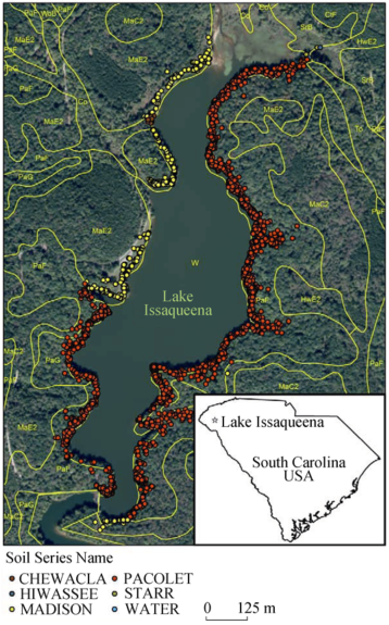
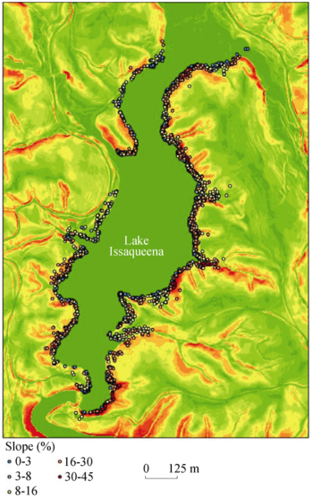
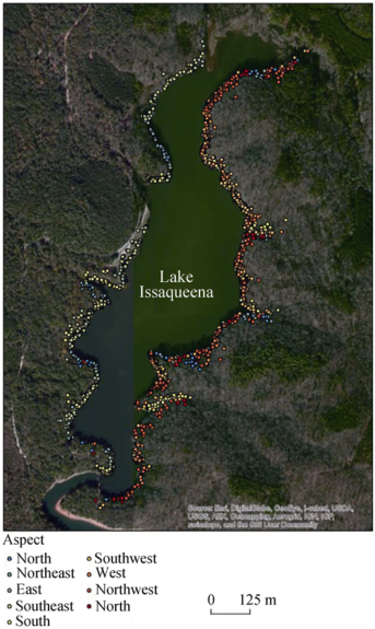
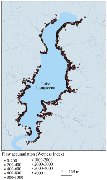
Spatio-temporal patterns of flowering in forest ecosystems are hard to quantify and monitor. The objectives of this study were to investigate spatio-temporal patterns (e.g. soils, simple slope classes, slope aspect, and flow accumulation) of flowering around Lake Issaqueena, South Carolina (SC, USA) using plant-flowering database collected with GPS- enabled camera (stored in Picasa 3 web albums and project website) on a monthly basis in 2012 and LiDAR-based topography. Pacolet fine sandy loam had the most flowering plants, followed by Madison sandy loam, both dominant soil types around the lake. Most flowering plants were on moderately steep (17%-30%) and gently sloping (4%-8%) slopes. Most flowering plants were on west (247.5°-292.5°), southwest (202.5°-247.5°), and northwest (292.5°-337.5°) aspects. Most flowering plants were associated with minimum and maximum flows within the landscape. Chi-square tests indicated differences in the distributions of the proportions of flowering plants were significant by soil type, slope, aspect, and flow accumulation for each month (February-November), for all months (overall), and across months. The Chi-square test on area-normalized data indicated significant differences for all months and individual differences by each month with some months not statistically significant. Cluster analysis on flowering counts for nine plant families with the most flowering counts indicated no unique separation by cluster, but implied that the majority of these families were flowering on strongly sloping (9%-16%) slopes, on southwest (202.5°-247.5°) aspects, and low flow accumulation (0-200). Presented methodology can serve as a template for future efforts to quantify spatio-temporal patterns of flowering and other phenological events.

Cite this article

HART Samantha , MIKHAILOVA Elena , POST Christopher , McMILLAN Patrick , SHARP Julia , BRIDGES William . Spatio-temporal analysis of flowering using
LiDAR topography[J]. Journal of Geographical Sciences, 2017
, 27(1) : 62 -78 . DOI: 10.1007/s11442-017-1364-x

1 Introduction

New technological advances are increasingly used to study and record phenological events, for example: remote sensing (Wei et al., 2014), digital repeat photography (Crimmins and Crimmins, 2008; Chen et al., 2011; Liang et al., 2012; Panchen, 2012; Nijland et al., 2013), website (Bradley et al., 2010), citizen science (Hill et al., 2012), and others. The majority of spatio-temporal studies on phenologies focused on agricultural crops and utilized remote sensing techniques (Chakaborty et al., 2014; Wei et al., 2014). However, Andrew and Ustin (2009) used a LiDAR based DEM to study the effects of microtypography and hydrology on the phenology of an invasive herb. Caillaud et al. (2010) modelled the spatial distribution and fruiting pattern for Dipteryx oleifera in Panama using a point process model of tree spatial distribution and a generalized linear mixed-effects model of temporal variation of fruit production. According to Dahlgren et al. (2007), environmental properties other than temperature, photoperiod, and moisture have not received much attention. Spatio-temporal patterns of flowering of a variety of plant species in forest ecosystems are hard to quantify and monitor because of the canopy cover, and there is a need to develop methodology for assessing phenology in such environments.
The majority of previous spatio-temporal studies on phenologies focused on agricultural crops and utilized remote sensing techniques, but such analysis is complicated in forested ecosystems. It is only in the last few years that LiDAR derived digital elevation models (DEMs) have become available. These LiDAR DEMs have sufficient horizontal and vertical accuracy to detect small changes in microtopography that had previously not been possible with coarser-scale spatial data. Additionally, the LiDAR DEMs use active remote sensing that is often able to penetrate forest canopy to see the underlying ground topography (Lorenzo Gil et al., 2013).
Flowering, one of many phenological events, occurs after a plant has transitioned from juvenile to adult and vegetative meristem buds change into a reproductive meristem, evocation (Gilbert, 2000). The transition of juvenile to adult occurs when the juvenile grows in size, age, and leaf number and has the right amount of water and light (photoperiod), and the right temperature (Gilbert, 2000). These factors cause a change in hormones, nutrient levels, and other chemicals (Gilbert, 2000). Plants flower at different times due to a variety of factors: pollinator availability, photoperiod (daily duration of light), temperature (thermoperiod), humidity, precipitation, and soil nutrients (especially phosphorus) (Lee and Amasino, 1995; Jones and Reithel, 2000; Gilbert, 2000; Evans, 2013a,b; Dahlgren et al., 2007; Jentsch et al., 2009).
Previous studies on the plant inventory and flowering around Lake Issaqueena in 1970-1971 (Pamplin, 1971) found 281 plants compared to 207 in 2011-2012 (Pamplin, 2013). Comparison of phenologies indicated 269 plant species blooming in 1970-1971 compared to 203 plants blooming in 2011-2012 (Pamplin, 1971, 2013). The blooming period was 11 months in 2011-2012 compared to 8 months in 1970-1971 (Pamplin, 1971, 2013). A majority of plants were blooming earlier and longer in 2011-2012 than in 1970-1971 (Pamplin, 1971, 2013).
The objectives of this study were to investigate spatio-temporal patterns (e.g. soils, simple slope classes, slope aspect, and flow accumulation) of flowering around Lake Issaqueena, SC using plant-flowering database collected with GPS-enabled camera and LiDAR topography.

2 Materials and methods

2.1 Study area

Lake Issaqueena (Figure 1) was built by the Works Progress Administration (WPA) in a Land Use Project introduced in 1934 that covered thousands of acres (Pamplin, 1971).
Lake Issaqueena is 116-acres in size, maintained by Issaqueena Dam in the northern part of Clemson Experimental Forest, and it was built for boating, swimming, and fishing. Clemson University acquired this land in 1954 and many research projects are undertaken within Clemson Experimental Forest (Pamplin, 1971).
Figure 1 Soil types and flowering occurrences around Lake Issaqueena, SC

2.2 Weather data

Long-term weather data were obtained from U.S. Historical Climatology Network- Monthly Data, Site 381770, Clemson University, South Carolina (Table 1).
Table 1 Monthly total precipitation (cm) and monthly average temperature (°C) for 2012, and 50-year mean (Source: U.S. Historical Climatology Network-Monthly Data, Site 381770, Clemson University, South Carolina)
2012 50-year mean
Month Mean temp., °C Precip., cm Mean temp.,°C Precip., cm
January 9 11 5 13
February 9 5 7 12
March 17 6 11 14
April 18 6 16 10
May 22 8 20 10
June 24 16 24 10
July 27 12 26 11
August 25 21 25 12
September 22 6 22 10
October 16 7 16 10
November 10 2 11 10
December 9 13 7 12
Total precip. 112 134
Mean temp. 17 16

2.3 Spatial analysis

A 3-m LiDAR derived DEM was obtained from Pickens County, SC and with an Issaqueena lake polygon from NHD USDS and an aerial photo of the study site from USDA-NRCS (Table 2; ESRI, 2013). The DEM is based on data acquired in 2011 at a 1.4 m point spacing with a horizontal accuracy of better than 1 m and a vertical accuracy of approximately 0.23 m. Slope was calculated using the ArcGIS 10.1 slope tool which reported the slope as the maximum rate of change in elevation of each 3.048 m by 3.048 m cell to its eight neighboring cells. Slopes were classified into simple slope classes based on definition and slope gradient limits defined by the Soil Survey Manual (2015) developed by United States Department of Agriculture and Natural Resources Conservation Service (USDA/NRCS). Aspect was found using the ArcGIS 10.1 aspect tool which identified the downslope direction of the maximum rate of change in elevation for each 3.048 m by 3.048 m cell. Flow accumulation was calculated using the ArcGIS 10.0 flow accumulation tool and was calculated as the number of cells expected to drain into each 3.048 m by 3.048 m cell.

2.4 Soil inventory

Soil map units were identified using Web Soil Survey (Table 2; Soil Survey Staff, 2015). The following soil types were identified around Lake Issaqueena: Chewacla soils, frequently flooded (Co) (Fine-loamy, mixed, active, thermic Fluvaquentic Dystrudepts); Hiwassee sandy loam, 10 to 25% slopes eroded (HwE2) (Very-fine, kaolinitic, thermic Rhodic Kanhapludults); Madison sandy loam, 10 to 25% slopes, eroded (MaE2) (Fine, kaolinitic, thermic Typic Kanhapludults); Pacolet fine sandy loam, 25 to 40% slopes (PaF) (Fine, kaolinitic, thermic Typic Kanhapludults); Pacolet fine sandy loam, 40 to 80% slopes (PaG) (Fine, kaolinitic, thermic Typic Kanhapludults); Rabun cobbly loam, 25 to 40% slopes (RaF) (Fine, kaolinitic, mesic Typic Kanhapludults); Starr loam, 0 to 6% slopes (SrB) (Fine-loamy, mixed, semiactive, thermic Fluventic Dystrudepts); Toccoa soils (To) (Coarse-loamy, mixed, active, nonacid, thermic Typic Udifluvents).
Table 2 Data sources and descriptions
Data layer Source Coordinate system Spatial resolution Date
DEM (LiDAR) Pickens County GIS NAD State Plane 1983 SC 3.048 m 2011
Lake Polygon NHD USGS NAD State Plane 1983 SC na 2013
NAIP Aerial Photo USDA-NRCS NAD State Plane 1983 SC 1 m 2013
SSURGO Soils Data USDA-NRCS Geographic na na

2.5 Floristic inventory, identification, and storage

Flowering plants were recorded via GPS enabled camera for future identification on a monthly basis. Flowering plants were identified using the USDA Plants Database (USDA, NRCS, 2014) and through the use of expert knowledge. Picasa 3 and Google Website were used to archive photos (Google, Inc., 2010).

2.6 Statistical analysis

Chi-square tests were used to examine the difference in distribution of proportions between flowering and soils, simple slope classes, slope aspects, and flow accumulations within each month, among the months, and overall when sample size was large enough to meet the assumptions. The Chi-square test was also performed using the normalized area percentages to examine the proportions within each month, among the months, and overall (SAS v. 9.3). Copyright, SAS Institute Inc. SAS and all other SAS Institute Inc. product or service names are registered trademarks or trademarks of SAS Institute Inc., Cary, NC, USA. Exploratory k-means cluster analysis was used to examine groups of slope classes, slope aspects, and flow accumulations by flowering families. Cluster analyses were performed using R Statistical Software (R Statistical Software, 2012).

3 Results and discussion

3.1 Soils and flowering

The Chi-square test (Table 3) indicated differences in the distribution of proportions of flowering counts among Chewacla, Madison, and Pacolet soil types were significant for all months (χ2(2)=4885.4, p=0.000) and for each individual month (p=0.000 for all tests, respectively). For the area-normalized data, the Chi-square test indicated that the differences in the distribution of proportions of flowering counts were significant over all months (χ2(2)=126.0, p=0.000), and for each individual month, significant differences were found in May (χ2(2)=53.5, p=0.000) and June (χ2(2)=71.5, p=0.000).
The soil series Pacolet fine sandy loam had the most flowering plants while Madison sandy loam had the second most (Figure 1 and Table 3). This is most likely due to the fact that Pacolet and Madison are the most dominant soil types in terms of area of the study site. Loam has been determined to be the best soil texture for agricultural crop growth (Brady and Weil 2004), and is the most conducive to plant growth around Lake Issaqueena. Chewacla, Starr loam and Hiawassee sandy loam soil series had very few flowering plants while Rabun cobbly loam and Toccoa had no flowering plants (Figure 1 and Table 3). The cobbly texture in the Rabun soil is problematic for retention of nutrients that would be beneficial to plant growth (USDA/NRCS, 2014). The Toccoa soil series had too small of an area in the study site to account for flowering plants.
Table 3 Flowering counts and area (m2 and %) by soil type around Lake Issaqueena, SC in 2012

3.2 Simple slope classes and flowering

The largest number of flowering plants was found on moderately steep slopes of 17%-30% followed by strong slopes of 9%-16% and gentle slopes of 4%-8% (Figure 2 and Table 4). The Chi-square test (Table 4), indicated that the differences in the distribution of proportions of flowering counts were significant for all months (χ2(4)=1905.6, p=0.000), across months (χ2(40)=232.2, p=0.000), and for each individual month March through November (p=0.000 for all tests, respectively). For the area-normalized data, the Chi-square test indicated that the differences in the distribution of proportions of flowering counts were significant over all months (χ2(4)=139.3, p=0.000), across months (χ2(59)=3176.8, p=0.000), and for each individual month, significant differences were found for all months examined except September (χ2(4)=8.5, p=0.075).
Figure 2 Simple slope classes and flowering occurrences around Lake Issaqueena, SC
Study by Komac et al. (2011) reported that plant expansion rates were faster on steeper slopes than shallow slopes. Steep slopes of 30%-45% and nearly level slopes of 0-3% had far fewer flowering plants than the other slopes with the exception of steep slopes of 45% and above (Figure 2 and Table 4). Andrew and Ustin (2009) reported an association between more mature phenology and shallower slopes. On the steepest slopes, there is less organic matter in the soil as it is washed down the slope gradient with the rain and less organic matter leaves fewer nutrients necessary for plants to flower (Corral-Nunez et al., 2014). On less steep slopes, plants can be in competition with grasses (Komac et al., 2011), and it may explain the fewer flowering plants found on the nearly level slopes.
Table 4 Flowering counts area(m2 and %) by simple slope classes (Soil Survey Manual,2015) around Lake Issaqueena, Sc in 2012

3.3 Slope aspect and flowering

The highest number of flowering plants was found on the western aspect, followed by southwestern and northwestern aspects (Figure 3 and Table 5). The next most productive slope aspects, in order of descending number of flowering plants were the southeastern, southern, and eastern aspects (Figure 3 and Table 5). The Chi-square test (Table 5) indicated that the differences in the distribution of proportions of flowering counts were significant for all months (χ2(8) =1141.1, p=0.000), across months (χ2(80)= 534.3, p=0.000), and for each individual month (p=0.000 for all tests). For the area- normalized data, the Chi-square test indicated that the differences in the distribution of proportions of flowering counts were significant over all months (χ2(8)=297.4, p=0.000), across months (χ2(107)=3997.1, p=0.000) and for each individual month, significant differences were found for all months examined except March (χ2(8)= 13.4, p=0.099).
It has been generally reported that south-facing aspects tend to be warmer and drier than north-facing slope aspects (Haase 1970). Dahlgren et al. (2007) reported that the flowering of Actaea spicata Linnaeus was earlier on south-facing slopes. Andrew and Ustin (2009) reported that the flowering of Lepidium latifolium Linnaeus was earlier on steeper north-facing slopes and that earlier flowering was more likely at higher eastness with the reverse being true in a lowland area.
Figure 3 Slope aspect and flowering occurrences around Lake Issaqueena, SC
Table 5 Flowering counts and area(m2 and %) by slope aspect around Lake Issaqueena, Sc in 2012

3.4 Flow accumulation and flowering

It has been reported that phenology stages occur earlier in dry years and later in wet years with the extent of the differentiation depending on site specific conditions and regional scale hydrology (Andrew and Ustin, 2009). The highest number of flowering plants was associated with minimum flow (dry areas) followed by those with maximum flow (wet areas) while flow levels in between had the least number of flowering plants (Figure 4 and Table 6).
Figure 4 Flow accumulation and flowering occurrences around Lake Issaqueena, SC
The Chi-square test (Table 6) indicated that the differences in the distribution of proportions were significant for all months (χ2(8)= 22586.5, p=0.000), and for each individual month examined (p=0.000 for each test). For the area-normalized analysis, the Chi-square test indicated that the differences in the distribution of proportions of flowering counts were significant over all months (χ2(8)=480.4, p=0.000). Small sample sizes prohibited the area-normalized analysis for each month.
Table 6 Flowering counts and area (m2 and %) by flow accumulation around Lake Issaqueena, Sc in 2012

3.5 Flowering patterns

Nine plant families with the most flowering counts were identified (number of flowering counts): Asteraceae (533), Fabaceae (299), Liliaceae (132), Melastomataceae (115), Ericaceae (105), Lamiaceae (101), Campanulaceae (97), Clusiaceae (84), and Caryophyllaceae (82) (Figures 5 and 6, Table 7). Cluster analysis (Table 8) on flowering counts for nine plant families with the most flowering counts indicated no unique separation by cluster, but indicated that a majority of these families were flowering on strongly sloping (9%-16%) slopes, on southwest (202.5°-247.5°) aspects, and low flow accumulation (0-200).
Within the most abundantly flowering family, Asteraceae (n=533), the most abundantly flowering species was Hieracium venosum Linnaeus (n=68), followed by Coreopsis major Linnaeus (n=60), and Coreopsis major Walter (n=60). Within the second most abundantly flowering family, Fabaceae (n=299), the most abundantly flowering species was Desmodium nudiflorum (Linnaeus) DC. (n=38), followed by Mimosa microphylla Dryant. (n=36), and Clitoria mariana Linnaeus (n=34).
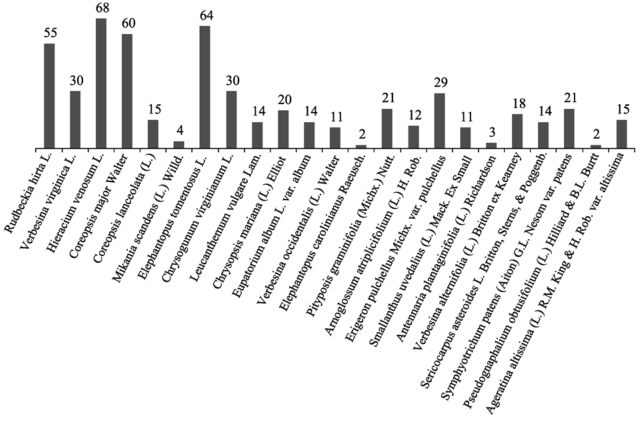
Figure 5 Flowering counts distribution within the Asteraceae family
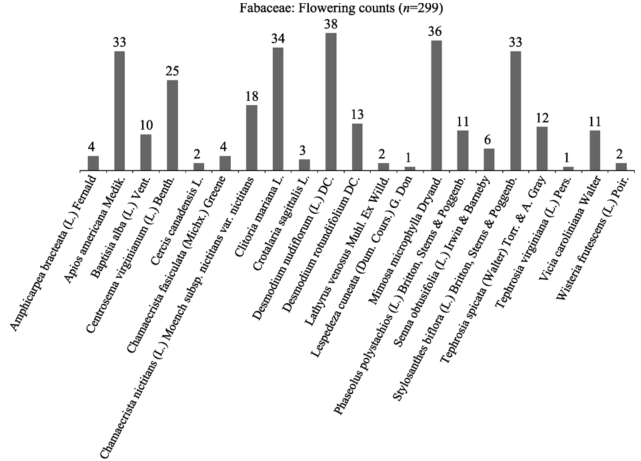
Figure 6 Flowering counts distribution within the Fabaceae family
Table 7 Landscape characteristics associated with the top nine families in terms of flowering counts around Lake Issaqueena, SC in 2012
Family Slope aspect Slope Flow accumulation
n Mean St dev. Mean St dev. Mean St dev.
Overall
Asteraceae 533 215.3 80.7 16 8 453 3392
Campanulaceae 97 180.0 97.8 14 10 223 777
Caryophyllaceae 82 229.7 93.5 19 8 448 1617
Clusiaceae 84 218.3 86.9 13 8 218 737
Ericaceae 105 249.1 80.6 18 11 293 1229
Fabaceae 304 183.6 82.7 16 8 758 6260
Lamiaceae 101 231.6 61.3 17 8 97 510
Liliaceae 132 243.4 94.9 17 8 79 276
Melastomataceae 115 192.7 78.5 11 8 2816 7502
February
Asteraceae 2 167.0 0.0 17 0 1 0
March
Asteraceae 52 212.9 88.9 18 9 103 257
Caryophyllaceae 26 210.6 83.7 18 8 104 313
Ericaceae 21 192.9 119.0 11 6 333 1003
Fabaceae 22 183.4 110.3 16 9 229 725
Lamiaceae 4 222.4 2.2 15 3 9 0
Liliaceae 36 222.8 116.0 16 6 46 185
April
Asteraceae 61 270.8 42.0 21 8 287 1395
Caryophyllaceae 10 265.9 33.2 17 7 1060 2308
Ericaceae 66 274.4 52.1 20 10 341 1443
Fabaceae 7 275.3 60.3 18 10 142 247
Lamiaceae 12 257.6 87.7 17 9 417 1393
Liliaceae 52 238.1 108.1 13 7 50 161
May
Asteraceae 64 224.4 80.8 13 8 231 695
Campanulaceae 8 125.2 21.3 27 4 9 4
Caryophyllaceae 12 309.3 34.6 22 10 950 3155
Ericaceae 7 257.1 19.4 23 7 5 7
Fabaceae 52 175.8 73.7 17 7 198 719
Lamiaceae 32 249.1 45.5 17 9 81 257
Liliaceae 8 283.4 38.2 18 8 313 378
Melastomataceae 6 123.4 36.1 7 8 2253 3092
June
Asteraceae 62 222.7 78.9 17 7 146 516
Campanulaceae 21 227.7 101.4 15 11 52 102
Caryophyllaceae 4 60.5 85.5 27 2 1 1
Clusiaceae 14 191.0 77.6 12 11 21 17
Ericaceae 3 181.7 138.4 25 3 38 9
Fabaceae 46 218.4 76.8 16 7 163 699
Lamiaceae 9 231.6 71.1 17 8 122 336
Liliaceae 16 244.5 43.4 20 10 6 6
Melastomataceae 28 215.6 79.0 11 7 5330 12178
July
Asteraceae 121 194.3 76.2 17 7 237 1541
Campanulaceae 11 163.4 135.8 9 5 3 2
Caryophyllaceae 22 232.0 101.2 18 7 417 1321
Clusiaceae 49 221.2 88.3 14 7 358 944
Ericaceae 5 244.8 37.0 18 15 11 4
Fabaceae 78 192.9 80.9 15 8 199 726
Lamiaceae 27 219.6 58.2 20 8 18 54
Liliaceae 8 264.4 49.2 30 3 6 5
Melastomataceae 52 187.6 81.7 11 9 2094 5130
August
Asteraceae 84 203.4 79.6 13 8 610 2147
Campanulaceae 43 161.2 90.0 13 9 419 1125
Caryophyllaceae 7 195.5 91.0 18 9 405 844
Clusiaceae 21 229.6 89.9 13 7 21 40
Fabaceae 89 162.0 78.0 14 8 2145 11447
Lamiaceae 16 199.1 62.8 13 6 40 93
Liliaceae 12 286.0 16.2 18 8 295 692
Melastomataceae 29 193.8 71.4 11 8 1802 5295
September
Asteraceae 36 195.1 92.5 14 8 1219 4083
Campanulaceae 9 221.6 75.1 14 5 8 7
Caryophyllaceae 1 273.7 NA 8 NA 39 NA
Fabaceae 8 122.3 15.7 26 4 12 8
Lamiaceae 1 236.5 NA 18 NA 1 NA
October
Asteraceae 37 224.3 72.0 17 9 1912 11277
Campanulaceae 5 190.6 91.4 22 9 471 420
Ericaceae 2 97.4 5.8 0 0 528 152
Fabaceae 2 104.9 31.6 11 9 2 2
Table 8 Cluster analysis for landscape characteristics associated with the top nine families in terms of flowering counts around Lake Issaqueena, SC in 2012
Cluster
1 2 3 4 5
Family
Asteraceae 8 14 510 0 1
Campanulaceae 0 5 92 0 0
Caryophyllaceae 1 5 76 0 0
Clusiaceae 0 3 81 0 0
Ericaceae 2 3 100 0 0
Fabaceae 3 12 282 1 1
Lamiaceae 0 1 100 0 0
Liliaceae 0 1 131 0 0
Melastomataceae 12 9 91 3 0
Parameter
Slope Aspect (°) 179 141 215 262 198
Simple Slope (%) 5 7 16 2 1
Flow Accumulation 12870 3260 57 41257 81820

4 Conclusions

This study examined the effects of environmental factors (soil type, slope class, slope aspect, and flow accumulation) on spatio-temporal patterns of flowering in forest ecosystems.
(1) The spatio-temporal analysis of flowering for all plants around Lake Issaqueena indicated significant differences in flowering by plant family, soil type, slope class, slope aspect, and flow accumulation for all months (p=0.000), across month (p=0.000), with the exception of flow accumulation across months (p=0.162). Area normalized differences in flowering by month for slope and slope aspect between March and October were significant (p=0.000) with the exception of September for slope (p=0.075), and March for slope aspect (p=0.099). This is new evidence that flowering is influenced by microtopography and soil type.
(2) A cluster analysis using flowering counts for the nine plant families with the highest flowering numbers indicated no unique separation by cluster, but implied that the majority of these families were flowering on strongly sloping (9%-16%) areas with southwest (202.5°-247.5°) aspects, and low flow accumulation (0-200). This shows a grouping of the most predominantly flowering plants in a particular slope, aspect and flow accumulation areas.
(3) The use of GPS-enabled camera, LiDAR derived data, and GIS are important tools for phenological studies and monitoring in forested ecosystems. As demonstrated with this study, it is now possible to analyze the relationship of slope, aspect, or predicted water flow to flowering because of the availability of more accurate ground topography represented by the LiDAR based DEMs. Although, the climate is expected to change at the rates exceeding geomorphological changes, the landscape characteristics are essential in identifying and protecting the “refugia” (habitats suitable for retreat, persistence, and potential expansion under changing environmental conditions).

The authors have declared that no competing interests exist.

[1]
Andrew M E, Ustin S L, 2009. Effects of microtypography and hydrology on phenology of an invasive herb.Ecography, 32: 860-870.Phenological traits may influence invasion success via effects on invasiveness of the colonizing species and invasibility of the receiving ecosystems. Many species exhibit substantial fine-scaled spatial variation in phenology and interannual differences in phenological timing in response to environmental variation. Yet describing and understanding this variation is limited by the availability of appropriate spatial and temporal datasets. Remote sensing provides such datasets, but has primarily been used to monitor broad-scale phenological patterns at coarse resolutions, necessarily missing fine spatial detail and intraspecies variation. We used hyperspectral remote sensing to characterize the spatial and temporal phenological variation of the invasive species Lepidium latifolium (perennial pepperweed) at two sites in California's San Francisco Bay/Sacramento芒聙聯San Joaquin River Delta. Considerable phenological variation was detected: L. latifolium was simultaneously present in vegetative, early flowering, peak flowering, fruiting, and senescent stages in late June; the relative dominance and distribution of these stages varied interannually. Environmental determinants of phenology were investigated with variables derived from the hyperspectral image data, from a high resolution LiDAR (light detection and ranging) digital elevation model (DEM), and from local precipitation and streamflow data. Lepidium latifolium phenology was found to track water availability, and may also be influenced by intraspecific competition and edaphic stress. Lepidium latifolium has a unique phenology (summer flowering) relative to the communities it invades, which may allow invasion of an empty niche. Furthermore, many habitats are invaded by L. latifolium, which occurs in locally appropriate phenologies under the different environmental conditions. The environmental responsiveness of L. latifolium phenology may mediate the wide breadth of invasible habitats.

DOI

[2]
Bradley E, Roberts D, Still C, 2010. Design of an image analysis website for phenological and meteorological monitoring.Environmental Modeling and Software, 25(1): 107-116.Web camera image databases and web-based services can be valuable components for a variety of modelling applications, but are still areas of relatively new exploration. Investigating design and information flow for an online image archive and analysis site for plant phenology and meteorological research has broader relevance to considerations of interoperability and website features. Currently, numerous online weather cameras provide images, but have no or limited-utility archives and do not support quantitative image analysis. We describe the design and implementation of a website ( http://zulu.geog.ucsb.edu/Data/camera.html) that both provides different display options for archived image review, as well as the ability to chart time-series values extracted for user-specified regions of interest. This interface is distinguished by content-enabled charts with the ability to click on data points and directly access the corresponding image for reference purposes. A linked website to the meteorological data from the camera station further extends the potential for exploratory analysis and pedagogical utility. Online quantification of the color change related to plant senescence and insolation impacts due to cloud cover are demonstrated. We conclude that dynamic web pages are a powerful and useful tool for adding educational and scientific value to repeat digital photography systems.

DOI

[3]
Brady N C, Weil R R, 2004. Elements of the Nature and Properties of Soils. 2nd ed. Pearson, Prentice Hall. Upper Saddle River, New Jersey 07458.ABSTRACT Incluye bibliografía e índice

[4]
Caillaud D, Crofoot M, Scarpino S,et al., 2010. Modeling the spatial distribution and fruiting pattern of a key tree species in a neotropical forest: Methodology and potential applications.PLOS ONE, 5(11): 1-10.The movement patterns of wild animals depend crucially on the spatial and temporal availability of resources in their habitat. To date, most attempts to model this relationship were forced to rely on simplified assumptions about the spatiotemporal distribution of food resources. Here we demonstrate how advances in statistics permit the combination of sparse ground sampling with remote sensing imagery to generate biological relevant, spatially and temporally explicit distributions of food resources. We illustrate our procedure by creating a detailed simulation model of fruit production patterns for Dipteryx oleifera, a keystone tree species, on Barro Colorado Island (BCI), Panama.Aerial photographs providing GPS positions for large, canopy trees, the complete census of a 50-ha and 25-ha area, diameter at breast height data from haphazardly sampled trees and long-term phenology data from six trees were used to fit 1) a point process model of tree spatial distribution and 2) a generalized linear mixed-effect model of temporal variation of fruit production. The fitted parameters from these models are then used to create a stochastic simulation model which incorporates spatio-temporal variations of D. oleifera fruit availability on BCI.We present a framework that can provide a statistical characterization of the habitat that can be included in agent-based models of animal movements. When environmental heterogeneity cannot be exhaustively mapped, this approach can be a powerful alternative. The results of our model on the spatio-temporal variation in D. oleifera fruit availability will be used to understand behavioral and movement patterns of several species on BCI.

DOI PMID

[5]
Chakraborty A, Seshasai M, Dadhwal V, 2014. Geo-spatial analysis of the temporal trends of kharif crop phenology metrics over India and its relationships with rainfall parameters. Environmental Monitoring and Assessment, 186: 4531-4542.The Global Inventory Modeling and Mapping Studies bimonthly Normalized Difference Vegetation Index (NDVI) data of 865×65802km spatial resolution for the period of 1982-2006 were analyzed to detect the trends of crop phenology metrics (start of the growing season (SGS), seasonal NDVI amplitude (AMP), seasonally integrated NDVI (SiNDVI)) during kharif season (June to October) and their relationships with the amount of rainfall and the number of rainy days over Indian subcontinent. Direction and magnitude of trends were analyzed at pixel level using the Mann-Kendall test and further assessed at meteorological subdivision level using field significance test (α65=650.1). Significant pre-occurrence of the SGS was observed over northern (Punjab, Haryana) and central (Marathwada, Vidarbha and Madhya Maharashtra) parts, whereas delay was found over southern (Rayalaseema, Coastal Andhra Pradesh) and eastern (Bihar, Gangetic West Bengal and Sub-Himalayan West Bengal) parts of India. North, west, and central India showed significant increasing trends of SiNDVI, corroborating the kharif food grain production performance during the time frame. Significant temporal correlation (α65=650.1) between the rainfall/number of rainy days and crop phenology metrics was observed over the rainfed region of India. About 35-4002% of the study area showed significant correlation between the SGS and the rainfall/number of rainy days during June to August. June month rainfall/number of rainy days was found to be the most sensitive to the SGS. The amount of rainfall and the number of rainy days during monsoon were found to have significant influence over the SiNDVI in 24-3002% of the study area. The crop phenology metrics had significant correlation with the number of rainy days over the larger areas than that of the rainfall amount.

DOI PMID

[6]
Chen H, Yin K, Wang H,et al., 2011. Detecting one-hundred-year environmental changes in western China using seven-year repeat photography.PLOS ONE, 6(9): 1-13.Due to its diverse, wondrous plants and unique topography, Western China has drawn great attention from explorers and naturalists from the Western World. Among them, Ernest Henry Wilson (1876 –1930), known as ‘Chinese’ Wilson, travelled to Western China five times from 1899 to 1918. He took more than 1,000 photos during his travels. These valuable photos illustrated the natural and social environment of Western China a century ago. Since 1997, we had collected E.H. Wilson's old pictures, and then since 2004, along the expedition route of E.H. Wilson, we took 7 years to repeat photographing 250 of these old pictures. Comparing Wilson's photos with ours, we found an obvious warming trend over the 100 years, not only in specific areas but throughout the entire Western China. Such warming trend manifested in phenology changes, community shifts and melting snow in alpine mountains. In this study, we also noted remarkable vegetation changes. Out of 62 picture pairs were related to vegetation change, 39 indicated vegetation has changed to the better condition, 17 for degraded vegetation and six for no obvious change. Also in these photos at a century interval, we found not only rapid urbanization in Western China, but also the disappearance of traditional cultures. Through such comparisons, we should not only be amazed about the significant environmental changes through time in Western China, but also consider its implications for protecting environment while meeting the economic development beyond such changes.

DOI PMID

[7]
Crimmins M, Crimmins T, 2008. Monitoring plant phenology using digital repeat photography.Environmental Management, 41: 949-958.Repeated observations of plant phenology have been shown to be important indicators of global change. However, capturing the exact date of key events requires daily observations during the growing season, making phenologic observations relatively labor intensive and costly to collect. One alternative to daily observations for capturing the dates of key phenologic events is repeat photography. In this study, we explored the utility of repeat digital photography for monitoring phenologic events in plants. We provide an illustration of this approach and its utility by placing observations made using repeat digital imagery in context with local meteorologic and edaphic variables. We found that repeat photography provides a reliable, consistent measurement of phenophase. In addition, digital photography offers advantages in that it can be mathematically manipulated to detect and enhance patterns; it can classify objects; and digital photographs can be archived for future analysis. In this study, an estimate of greenness and counts of individual flowers were extracted by way of mathematic algorithms from the photo time series. These metrics were interpreted using meteorologic measurements collected at the study site. We conclude that repeat photography, coupled with site-specific meteorologic measurements, could greatly enhance our understanding environmental triggers of phenologic events. In addition, the methods described could easily be adopted by citizen scientists and the general public as well as professionals in the field.

DOI PMID

[8]
Dahlgren J P, von Zeipel H, Ehrlen J, 2007. Variation in vegetative and flowering phenology in a forest herb caused by environmental heterogeneity.American Journal of Botany, 94(9): 1570-1576.Timing of seasonal plant development can affect biotic interactions and plant fitness. Phenology is governed largely by temperature and may therefore be affected by global climate warming, making this an important area of research. Several factors in addition to temperature may cause differences in phenology. We studied the influence of local environment, plant size, and reproductive effort on shoot emergence and flowering time of 290 individuals of Actaea spicata (Ranunculaceae), distributed among 25 plots in four populations. We used multiple regression and structural equation models (SEM) to study causal relationships. Among plots, soil temperature and canopy cover explained 63% of the variation in shoot emergence. Soil temperature, slope, and canopy cover together explained 83% of the variation in flowering time. Within plots, small plants on steep south-facing slopes with high soil potassium concentrations emerged earlier in the year. Plants emerging earlier flowered earlier, but no environmental factors affected flowering time directly. We found no effects of reproductive effort. Our results support the view that flowering time of temperate forest herbs is constrained by several environmental factors acting indirectly through effects on shoot emergence time.

DOI PMID

[9]
ESRI, 2013. ArcGIS Desktop: Release 10.2 Redlands, CA: Environmental Systems Research Institute.

[10]
Evans E, 2013a. Action Mode, Deficiency, and Toxicity Symptoms of the 17 Essential Nutrients. Nutrient Deficiency. North Carolina State University College of Ag. and Life Sciences Cooperative Extension.

[11]
Evans E, 2013b. Temperature Effect on Plants. Horticultural Science. NC State University College of Ag. and Life Sciences Cooperative Extension.Glavni izvor topline na Zemlji je Sunce. Temperatura je samo indikator toplinskog stanja. Atmosfera se zagrijava toplinskom radijacijom kopna i mora, jer sun00evo zra00enje prolazi kroz atmosferu a da je prakti00ki ne zagrijava. Aktivna povr08ina prima globalno zra00enje i protuzra00enje atmosfere, koje najve04im dijelom upija, te se zbog toga zagrijava. Kada je rije00 o temperaturama mo06e se govoriti o: -optimalnim -kardinalnim - kriti00nim temperaturama. Optimalne su one pri kojima se vitalne funkcije biljaka odvijaju maksimalnom brzinom, gledano integralno u biljci. Kardinalne temperature, minimalne i maksimalne su pak one ispod ili iznad kojih prestaju 06ivotne funkcije, ali se eventualno mogu povratiti ako se uvjeti pobolj08aju. Kriti00ne temperature su one minimalne i maksimalne temperature ispod ili iznad kojih se javljaju nepopravljive 08tete u funkcijama ili na biljnim organima. Jo08 treba dodati tzv. 67biolo08ki temperaturni minimum“ 08to predstavlja donju granicu 06ivota, ali samo kad prestaje aktivan rast, a stanica nije uginula. On je razli00it za pojedine kulture i da bi se mogao shvatiti treba najprije podijeliti kulture prema zahtjevima za temperaturama, i to: 1. Skupina termofilnih kultura 00iji je aktivni 06ivot pomaknut u zonu vi08ih temperatura, temperaturni prag im je u pravilu iznad 5 °C 2. Kriofilne kulture se dobro prilago04avaju i niskim temperaturama, ili 00ak za svoj rast i razvoj tra06e period niskih temperatura. Glede optimalnih, minimalnih i maksimalnih temperatura, u 08irokom prosjeku se ra00una na raspon od 0-45 °C. Izme04u 25 i 30 °C je prosje00an optimum za ve04inu fiziolo08kih procesa, osobito za fotosintezu. Maksimum za primanje vode le06i izme04u 35 i 40 °C. Optimum disanja je izme04u 36 i 40 °C. Pri 45 °C inaktivira se klorofil i prestaje fotosinteza. Na 50 °C prestaje disanje. Optimum za cvatnju i oplodnju je oko 25 °C a za sazrijevanje vi08e od 25 °C. Pri djelovanju niskih temperatura disanje prestaje pri -10 °C, iako neke kulture podnose i od -38 do – 40 °C ( kru08ka i jabuka )

[12]
Gilbert S, 2000. Developmental Biology. 6th ed. Sunderland:Sinauer Associates. 222-227.

[13]
Google, Inc., 2010. Picasa Web Albums Data API for .NET (Version 1.0). Mountain View, CA. Available at

[14]
Haase E F, 1970. Environmental fluctuations on south-facing slopes in the Santa Catalina Mountains of Arizona.Ecology, 51(6): 959-974.Solar radiation, evaporation, air- and soil-temperature extremes, soil moisture, and precipitation were measured on four aspects (SSE, S, SSW, SW) of constant slope in the desert foothills of the Santa Catalina Mountains over a 1-year period. The sequence of warmest and driest aspects based upon annual means was S, SSW, SW, SSE. The warmest and driest aspect may change with the environmental factor considered or the time of year. Drought extremes reached a high peak on the SW aspect during the arid spring, although during all other seasons the SW aspect had the mildest drought conditions. The warmest and driest aspect during the summer rainy season was SSE, during the winter rainy season it was S, and during the fall arid season S and SSE were nearly equal. Few significant differences were found throughout the year between S and SSW aspects. When vegetation and environment are considered, the warmest and driest aspect may also change with the species because plants may utilize different microenvironments at different seasons and vary in their response to similar environmental changes.

DOI

[15]
Hill A, Guralnick R, Smith A,et al., 2012. The notes from nature tool for unlocking biodiversity records through citizen science.Zoo Keys, 209: 219-233.Legacy data from natural history collections contain invaluable and irreplaceable information about biodiversity in the recent past, providing a baseline for detecting change and forecasting the future of biodiversity on a human-dominated planet. However, these data are often not available in formats that facilitate use and synthesis. New approaches are needed to enhance the rates of digitization and data quality improvement. Notes from Nature provides one such novel approach by asking citizen scientists to help with transcription tasks. The initial web-based prototype of Notes from Nature is soon widely available and was developed collaboratively by biodiversity scientists, natural history collections staff, and experts in citizen science project development, programming and visualization. This project brings together digital images representing different types of biodiversity records including ledgers , herbarium sheets and pinned insects from multiple projects and natural history collections. Experts in developing web-based citizen science applications then designed and built a platform for transcribing textual data and metadata from these images. The end product is a fully open source web transcription tool built using the latest web technologies. The platform keeps volunteers engaged by initially explaining the scientific importance of the work via a short orientation, and then providing transcription 鈥渕issions鈥 of well defined scope, along with dynamic feedback, interactivity and rewards. Transcribed records, along with record-level and process metadata, are provided back to the institutions. While the tool is being developed with new users in mind, it can serve a broad range of needs from novice to trained museum specialist. Notes from Nature has the potential to speed the rate of biodiversity data being made available to a broad community of users.

DOI PMID

[16]
Jentsch A, Kreyling J, Boettcher-Treschkow J,et al., 2009. Beyond gradual warming: Extreme weather events alter flower phenology of European grassland and heath species.Global Change Biology, 15: 837-849.Shifts in the phenology of plant and animal species or in the migratory arrival of birds are seen as 'fingerprints' of global warming. However, even if such responses have been documented in large continent-wide datasets of the northern hemisphere, all studies to date correlate the phenological pattern of various taxa with gradual climatic trends. Here, we report a previously unobserved phenomenon: severe drought and heavy rain events caused phenological shifts in plants of the same magnitude as one decade of gradual warming. We present data from two vegetation periods in an experimental setting containing the first evidence of shifted phenological response of 10 grassland and heath species to simulated 100-year extreme weather events in Central Europe. Averaged over all species, 32 days of drought significantly advanced the mid-flowering date by 4 days. The flowering length was significantly extended by 4 days. Heavy rainfall (170 mm over 14 days) had no significant effect on the mid-flowering date. However, heavy rainfall reduced the flowering length by several days. Observed shifts were species-specific, (e.g. drought advanced the mid-flowering date for Holcus lanatus by 1.5 days and delayed the mid-flowering date for Calluna vulgaris by 5.7 days, heavy rain advanced mid-flowering date of Lotus corniculatus by 26.6 days and shortened the flowering length of the same species by 36.9 days). Interestingly, the phenological response of individual species was modified by community composition. For example, the mid-flowering date of C. vulgaris was delayed after drought by 9.3 days in communities composed of grasses and dwarf shrubs compared with communities composed of dwarf shrubs only. This indicates that responses to extreme events are context specific. Additionally, the phenological response of experimental communities to extreme weather events can be modified by the functional diversity of a stand. Future studies on phenological response patterns related to climate change would profit from explicitly addressing the role of extreme weather events.

DOI

[17]
Jones K, Reithel J, 2000. Pollinator-mediated selection on a flower color polymorphism in experimental populations ofAntirrhinum(Scrophulariaceae). American Journal of Botany, 88(3): 447-454.We quantified pollinator visit behavior, pollen receipt and export, and changes in allele and genotype frequencies from initial Hardy- Weinberg conditions in experimental arrays of two color morphs of snapdragons (Antirrhinum majus) visited by freely foraging bumble bees (Bombus appositus and B. flavifrons). The number of pollen grains received by a flower depended most on the number of pollinator visits to the flower, whereas the number of grains exported was best predicted by the total time pollinators spent inside the flower. The pattern of mating generally was assortative with respect to color, as bees tended to overvisit one color or the other within a foraging bout. In arrays where nectar was augmented in one color, the augmented color received both more visits and longer visits. Allele and genotype frequencies in offspring samples were in accord with qualitative expectations based on the pollinator observations, demonstrating that pollinators can directly influence the evolution of single-locus floral traits, at least under simplified experimental conditions.

DOI PMID

[18]
Komac B, Alados C L, Camarero J J, 2011. Influence of topography on the colonization of subalpine grasslands by Thorny Cushion Dwarf (Echinospartum horridum). Arctic, Antarctic, and Alpine Research, 43(4): 601-611.

[19]
Liang L, Schwartz M, Fei S, 2012. Photographic assessment of temperate forest understory phenology in relation to springtime meteorological drivers.International Journal of Biometerology, 56(2): 343-355.Phenology shows sensitive responses to seasonal changes in atmospheric conditions. Forest understory phenology, in particular, is a crucial component of the forest ecosystem that interacts with meteorological factors, and ecosystem functions such as carbon exchange and nutrient cycling. Quantifying understory phenology is challenging due to the multiplicity of species and heterogeneous spatial distribution. The use of digital photography for assessing forest understory phenology was systematically tested in this study within a temperate forest during spring 2007. Five phenology metrics (phenometrics) were extracted from digital photos using three band algebra and two greenness percentage (image binarization) methods. Phenometrics were compared with a comprehensive suite of concurrent meteorological variables. Results show that greenness percentage cover approaches were relatively robust in capturing forest understory green-up. Derived spring phenology of understory plants responded to accumulated air temperature as anticipated, and with day-to-day changes strongly affected by estimated moisture availability. This study suggests that visible-light photographic assessment is useful for efficient forest understory phenology monitoring and allows more comprehensive data collection in support of ecosystem/land surface models.

DOI PMID

[20]
Lee I, Amasino R, 1995. Effect of vernalization, photoperiod, and light quality on the flowering phenotype of Arabidopsis plants containing the FRIGIDA gene.Plant Physiology, 108(1): 157-162.

[21]
Lorenzo Gill A, NunezCasillas L, Isenburg M,et al., 2013. A comparison between LiDAR and photogrammetry digital terrain models in a forest area on Tenerife Island.Canadian Journal of Remote Sensing, 39(5): 396-409.This paper compares two types of digital terrain models (DTMs) with ground elevation measures collected through field work in a dense forest area on the island of Tenerife (Canary Islands, Spain). The first was an existing DTM derived from altimetric features obtained by manual photogrammetric restitution. The second DTM was computed from aerial LiDAR data with a nadir density of 0.8 points00·m0908082. Both DTMs have a pixel size of 5 m. The field work consisted of measuring three elevation profiles by land surveying techniques using a total station survey and taking into account different vegetation covers. The analysis of the profiles by means of nonparametric techniques showed an accuracy at the 95th percentile between 0.54 m and 24.26 m for the photogrammetry-derived DTM and between 0.22 m and 3.20 m for the LiDAR-derived DTM. Plotting the elevation profiles allowed for the visual detection of locations where the models failed. The LiDAR data were able to reflect more accurately the true ground surface in areas of dense vegetation, especially in places where the ground was invisible to photogrammetric operators as in the case of Canarian pine forest with understory.

DOI

[22]
Nijland W, Coops N, Coogan S,et al., 2013. Vegetation phenology can be captured with digital repeat photography and linked to variability of root nutrition inHedysarum alpinum. Applied Vegetation Science, 16: 317-324.Question Can repeat (time-lapse) photography be used to detect the phenological development of a forest stand, and linked to temporal patterns in root nutrition for Hedysarum alpinum (alpine sweetvetch) an important grizzly bear food species? Location Eastern foothills and front ranges of the Rocky Mountains in Alberta, Canada. The area contains a diverse mix of mature and young forest, wetlands and alpine habitats. Methods We deployed six automated cameras at three locations to acquire daily photographs at the plant and forest stand scales. Plot locations were also visited on a bi-weekly basis to record the phenological stage of H.alpinum and other target plant species, as well as to collect a root sample for determination of crude protein content. Results Repeat photography and image analysis successfully detected all key phenological events (i.e. green-up, flowering, senescence). Given the relation between phenology and root nutrition, we illustrate how camera data can be used to predict the spatial and temporal distribution and quality of a key wildlife resource. Conclusions Repeat photography provides a cost-effective method for monitoring vegetation development, food availability, and nutritional quality at a forest stand scale. Since wildlife responds to the availability and quality of their food resources, detailed information on changes in resource availability helps with land-use management decisions and furthers our understanding of grizzly bear feeding ecology and habitat selection.

DOI

[23]
Pamplin W B, 1971. A floristic study of Lake Issaqueena. Master Thesis, Clemson University.

[24]
Pamplin R P, 2013. Multitemporal floristic and phenological (flowering) analysis of the shores of Lake Issaqueena, South Carolina [D]. Clemson University.

[25]
Panchen Z, Primack R, Anisko T,et al., 2012. Herbarium specimens, photographs, and field observations show Philadelphia area plants are responding to climate change.American Journal of Botany, 99(4): 751-756.The global climate is changing rapidly and is expected to continue changing in coming decades. Studying changes in plant flowering times during a historical period of warming temperatures gives us a way to examine the impacts of climate change and allows us to predict further changes in coming decades. The Greater Philadelphia region has a long and rich history of botanical study and documentation, with abundant herbarium specimens, field observations, and botanical photographs from the mid-1800s onward. These extensive records also provide an opportunity to validate methodologies employed by other climate change researchers at a different biogeographical area and with a different group of species.Data for 2539 flowering records from 1840 to 2010 were assessed to examine changes in flowering response over time and in relation to monthly minimum temperatures of 28 Piedmont species native to the Greater Philadelphia region.Regression analysis of the date of flowering with year or with temperature showed that, on average, the Greater Philadelphia species studied are flowering 16 d earlier over the 170-yr period and 2.7 d earlier per 1掳C rise in monthly minimum temperature.Of the species studied, woody plants with short flowering duration are the best indicators of a warming climate. For monthly minimum temperatures, temperatures 1 or 2 mo prior to flowering are most significantly correlated with flowering time. Studies combining herbarium specimens, photographs, and field observations are an effective method for detecting the effects of climate change on flowering times.

DOI PMID

[26]
R Statistical Software, 2012. R: A Language and Environment for Statistical Computing. R Core Development Team. Vienna, Austria.

[27]
SAS v. 9.3, 2011. Copyright, SAS Institute Inc. SAS and all other SAS Institute Inc. product or service names are registered trademarks or trademarks of SAS Institute Inc., , Cary, NCUSA.

[28]
Soil Survey Manual, 2015. Natural Resources Conservation Service, United States Department of Agriculture. Soil Slope. Available online at [10/15/15].

[29]
Soil Survey Staff, 2015. Natural Resources Conservation Service, United States Department of Agriculture. Web Soil Survey. Available online at [10/15/15].

[30]
USDA, NRCS, 2014. The PLANTS Database (, 28 January 2014). National Plant Data Team, Greensboro, NC 27401-4901 USA.

[31]
Wei G, Xiangnan N, Duanyang J, Shuheng L, 2014. Spatial-temporal patterns of vegetation dynamics and their relationships to climate variations in Qinghai Lake Basin using MODIS time-series data.Journal of Geographical Sciences, 24(6): 1009-1021.Global warming has led to significant vegetation changes in recent years. It is necessary to investigate the effects of climatic variations (temperature and precipitation) on vegetation changes for a better understanding of acclimation to climatic change. In this paper, we focused on the integration and application of multi-methods and spatial analysis techniques in GIS to study the spatio-temporal variation of vegetation dynamics and to explore the vegetation change mechanism. The correlations between EVI and climate factors at different time scales were calculated for each pixel including monthly, seasonal and annual scales respectively in Qinghai Lake Basin from the year of 2001 to 2012. The primary objectives of this study are to reveal when, where and why the vegetation change so as to support better understanding of terrestrial response to global change as well as the useful information and techniques for wise regional ecosystem management practices. The main conclusions are as follows: (1) Overall vegetation EVI in the region increased 6% during recent 12 years. The EVI value in growing seasons (i.e. spring and summer) exhibited very significant improving trend, accounted for 12.8% and 9.3% respectively. The spatial pattern of EVI showed obvious spatial heterogeneity which was consistent with hydrothermal condition. In general, the vegetation coverage improved in most parts of the area since nearly 78% pixel of the whole basin showed increasing trend, while degraded slightly in a small part of the area only. (2) The EVI change was positively correlated with average temperature and precipitation. Generally speaking, in Qinghai Lake Basin, precipitation was the dominant driving factor for vegetation growth; however, at different time scale its weight to vegetation has differences. (3) Based on geo-statistical analysis, the autumn precipitation has a strong correlation with the next spring EVI values in the whole region. This findings explore the autumn precipitation is an important indicator, and then, limits the plant growth of next spring.

DOI

Outlines

/