
Journal of Geographical Sciences >
Mapping the hotspots and coldspots of ecosystem services in conservation priority setting
Author: Li Yingjie (1990-), specialized in environmental change and ecosystem services. E-mail: lyj@snnu.edu.cn
*Corresponding author: Zhang Liwei (1985-), Assistant Professor, specialized in landscape ecology and ecosystem services. E-mail: zlw@snnu.edu.cn
Received date: 2016-03-15
Accepted date: 2016-07-29
Online published: 2017-06-10
Supported by
National Natural Science Foundation of China, No.41601182
National Social Science Foundation of China, No.14AZD094
National Key Research and Development Plan of China, No.2016YFC0501601
China Postdoctoral Science Foundation, No.2016M592743
Fundamental Research Funds for the Central Universities, No.GK201603078
Key Project of the Ministry of Education of China, No.15JJD790022
Copyright
Spatial-explicitly mapping of the hotspots and coldspots is a vital link in the priority setting for ecosystem services (ES) conservation. However, little research has identified and tested the compactness and efficiency of their ES hotspots and coldspots, which may weaken the effectiveness of ecological conservation. In this study, based on the RUSLE model and Getis-Ord Gi* statistics, we quantified the variation of annual soil conservation services (SC) and identified the statistically significant hotspots and coldspots in Shaanxi Province of China from 2000 to 2013. The results indicate that, 1) areas with high SC presented a significantly increasing trend as well, while areas with low SC only changed slightly; 2) SC hotspots and coldspots showed an obvious spatial differentiation—the hotspots were mainly spatially aggregated in southern Shaanxi, while the coldspots were mainly distributed in the Guanzhong Basin and Sand-windy Plateau; and 3) the identified hotspots had the highest capacity of providing SC, with 29.6% of the total area providing 59.7% of the total service. In contrast, the coldspots occupied 46.3% of the total area, but only provided 17.2% of the total SC. In addition to conserving single ES, the Getis-Ord Gi* statistics method can also help identify multi-functional priority areas for conserving multiple ES and biodiversity.
LI Yingjie , ZHANG Liwei , YAN Junping , WANG Pengtao , HU Ningke , CHENG Wei , FU Bojie . Mapping the hotspots and coldspots of ecosystem services in conservation priority setting[J]. Journal of Geographical Sciences, 2017 , 27(6) : 681 -696 . DOI: 10.1007/s11442-017-1400-x
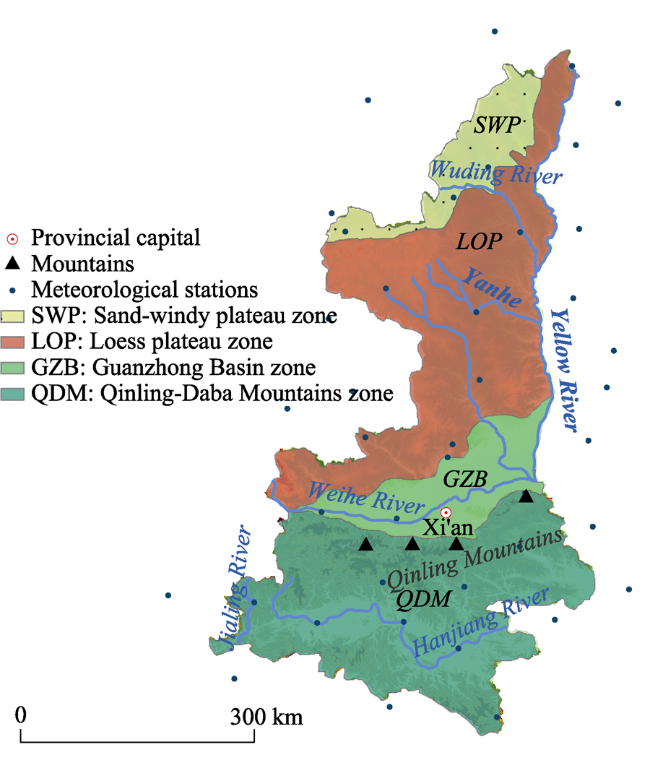
Figure 1 Location of meteorological stations and geographical division in Shaanxi Province, China |
Table 1 The datasets sources |
| Data | Type | Resolution | Time period | Sources |
|---|---|---|---|---|
| Meteorological data | Point | — | 2000-2013 | http://cdc.cma.gov.cn/ |
| Soil properties | Raster | 1 km | 2000 | http://webarchive.iiasa.ac.at/ |
| DEM | Raster | 90 m | 2004 | http://srtm.csi.cgiar.org/ |
| LULC | Polygon | 30 m | 2000, 2013 | http://www.landcover.org/data/ |
| MODIS NDVI | Raster | 250 m | 2000-2013 | http://ladsweb.nascom.nasa.gov/data/ |
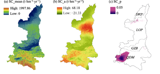
Figure 2 Spatial patterns of SC (a), change rate of SC (b) and the significant (P<0.05) change areas (c) from 2000 to 2013. The change rate at cell level was calculated by using the least square method (LSM). |
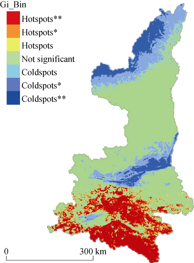
Figure 3 Hotspots and coldspots with different confidence levels (The double star (**) and single star (*) superscript indicate hotspots or coldspots are significant at 99% and 95% level respectively) |
Table 2 Statistics on the hotspots and coldspots of soil conservation service in Shaanxi Province, China |
| Annual SC per unit area (t·hm-2·a-1) | Area percentage (%) | Annual SC percentage (%) | |
|---|---|---|---|
| Coldspots** | 80.85 | 41.40 | 13.61 |
| Coldspots* | 175.99 | 4.95 | 3.55 |
| Coldspots | 190.68 | 2.41 | 1.87 |
| Not Significant | 239.34 | 20.63 | 20.08 |
| Hotspots | 296.79 | 1.02 | 1.24 |
| Hotspots* | 309.95 | 1.86 | 2.34 |
| Hotspots** | 508.08 | 27.73 | 57.31 |
Note: The double star (**) and a single star (*) superscript indicate hotspots or coldspots are significant at 99% and 95% level, respectively. |
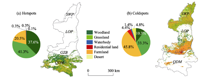
Figure 4 LULC types in hotspots and coldspots. The pie charts indicate the percentage of each LULC from the total area of hotspots or coldspots. |
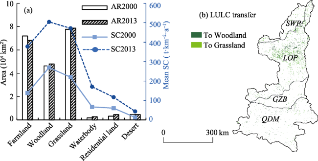
Figure 5 Comparison of LULC change between 2000 and 2013: (a) the area (AR) of LULC change and the mean SC provided by each LULC type; (b) the distribution of other types of LULC transferred to woodland and grassland |
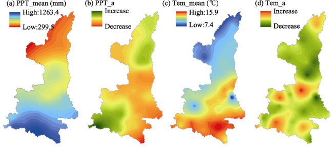
Figure 6 Spatial patterns of mean annual precipitation (PPT) (a), temperature (Tem) (c) and their change rates (b and d) from 2000 to 2013. The change rate at grid cell level was calculated by using the least square method (LSM). |
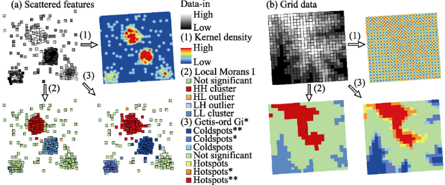
Figure 7 Comparison of three hotspot analysis methods: KDE (1), Local Moran’s I (2), Getis-Ord Gi* statistics (3)Note: When input features are spatially scattered (see Figure 7a), the KDE can only identify spatial cluster, but it mixes the cluster of high values (i.e., hotspots) and the cluster of low values (coldspots); that is, the KDE can neither tell what the cluster is nor whether it is significant. Fortunately, the Local Moran’s I and Getis-Ord Gi* statistics can both make it. The difference is that the Local Moran’s I is more efficient at identifying the outliers (see Figure 7a-(2) above), while the Gi* statistics is even better at identifying statistically significant hotspots and coldspots with different confidence levels (see Figure 7a-(3)). When input features are spatially uniform grid data (see Figure 7b), the KDE becomes inefficient, while the Local Moran’s I and Gi* statistics work well in this case, and the Gi* statistics especially holds its unique superiority. |
The authors have declared that no competing interests exist.
| [1] |
|
| [2] |
|
| [3] |
|
| [4] |
|
| [5] |
|
| [6] |
|
| [7] |
|
| [8] |
|
| [9] |
|
| [10] |
|
| [11] |
|
| [12] |
|
| [13] |
|
| [14] |
|
| [15] |
ESRI, 2013. ArcGISDesktop: Release 10.2. Redmond, CA: Esri Inc.
|
| [16] |
|
| [17] |
|
| [18] |
|
| [19] |
|
| [20] |
|
| [21] |
|
| [22] |
|
| [23] |
|
| [24] |
|
| [25] |
|
| [26] |
|
| [27] |
|
| [28] |
|
| [29] |
|
| [30] |
|
| [31] |
|
| [32] |
|
| [33] |
|
| [34] |
|
| [35] |
MA [Millenium Ecosystem Assessment], 2005. Ecosystems and Human Well-Being: Current State and Trends. Washington, DC Island Press.
|
| [36] |
|
| [37] |
|
| [38] |
|
| [39] |
|
| [40] |
|
| [41] |
|
| [42] |
|
| [43] |
|
| [44] |
|
| [45] |
|
| [46] |
|
| [47] |
|
| [48] |
|
| [49] |
|
| [50] |
|
| [51] |
|
| [52] |
|
| [53] |
|
| [54] |
|
| [55] |
|
| [56] |
|
| [57] |
|
| [58] |
|
| [59] |
|
| [60] |
|
/
| 〈 |
|
〉 |