Orginal Article

Location patterns of urban industry in Shanghai and implications for sustainability

  • CAO Weidong , 1 ,
  • LI Yingying 1, * ,
  • CHENG Jianquan , 2, 3 ,
  • Steven MILLINGTON 3
Expand
  • 1. College of Territorial Resources and Tourism, Anhui Normal University, Wuhu 241003, Anhui, China
  • 2. Key Laboratory of Beibu Gulf Environmental Change and Resources Utilization under Ministry of Education, Guangxi Teachers Education University, Nanning 530001, China
  • 3. School of Science and the Environment, Manchester Metropolitan University (MMU) Chester Street, Manchester, M1 5GD, UK

Author: Cao Weidong, PhD and Professor, specialized in industrial geography. E-mail: ;

*Corresponding author: Cheng Jianquan, E-mail:

Received date: 2016-11-22

  Accepted date: 2017-01-22

  Online published: 2017-07-10

Supported by

National Natural Science Foundation of China, No.41571124

Copyright

Journal of Geographical Sciences, All Rights Reserved

Abstract

China’s economy has undergone rapid transition and industrial restructuring. The term “urban industry” describes a particular type of industry within Chinese cities experiencing restructuring. Given the high percentage of industrial firms that have either closed or relocated from city centres to the urban fringe and beyond, emergent global cities such as Shanghai, are implementing strategies for local economic and urban development, which involve urban industrial upgrading numerous firms in the city centre and urban fringe. This study aims to analyze the location patterns of seven urban industrial sectors within the Shanghai urban region using 2008 micro-geography data. To avoid Modifiable Areal Unit Problem (MAUP) issue, four distance-based measures including nearest neighbourhood analysis, Kernel density estimation, K-function and co-location quotient have been extensively applied to analyze and compare the concentration and co-location between the seven sectors. The results reveal disparate patterns varying with distance and interesting co-location as well. The results are as follows: the city centre and the urban fringe have the highest intensity of urban industrial firms, but the zones with 20-30 km from the city centre is a watershed for most categories; the degree of concentration varies with distance, weaker at shorter distance, increasing up to the maximum distance of 30 km and then decreasing until 50 km; for all urban industries, there are three types of patterns, mixture of clustered, random and dispersed distribution at a varied range of distances. Consequently, this paper argues that the location pattern of urban industry reflects the stage-specific industrial restructuring and spatial transformation, conditioned by sustainability objectives.

Cite this article

CAO Weidong , LI Yingying , CHENG Jianquan , Steven MILLINGTON . Location patterns of urban industry in Shanghai and implications for sustainability[J]. Journal of Geographical Sciences, 2017 , 27(7) : 857 -878 . DOI: 10.1007/s11442-017-1410-8

1 Introduction

The recognition of the importance of industrial agglomeration to urban and regional economic development is not new. Marshall (1890), for example, described how firms operating within the same industry displayed a tendency to locate close to each other based on observations of the textiles industry in the 19th century Lancashire. In the post-war period, the notion of agglomeration reappeared within normative neo-classical location theories, which attempted to link firm location to exogenous factors including transport, land availability, tax and tariff rates, and market size, with a goal of achieving maximum profits (Yuan et al., 2014). The ‘new economic geography’ (or spatial economy theory), initiated by Krugman (1991a, 1991b), highlights the interactions between the two forces or processes: agglomeration and dispersion. The former includes economies of scale and transport costs and the latter mainly immobile workers, product market competition, and congestion. The location of industry is highly dependent on the outcomes of these interactions (Fujita et al., 1999).
Despite the overwhelming focus on western examples, interest in agglomeration economies now extends across the developing world, focusing in particular in areas experiencing rapid industrial restructuring, such as China (Hu et al., 2015; Pan and Xia, 2014; Fand and Liu, 2009). Since the economic reform initiated in 1978, China has achieved an unprecedented speed of urban and industrial development to become the second largest national economy by 2010. The composition of labour force in secondary industry increased continuously from 7.4% in 1952 to a peak of 27.2% in 2008 (Chen et al., 2011). As Chinese cities transform to post-socialism, China’s economic transition, namely globalization, marketization and decentralization, are also experiencing dramatic and continuing structural changes, and now shifting to a mix of heavy, light and high-tech industries (Ma et al., 2013). The persistence of a dual economic system may have contributed to the high concentration of industry during the current phase (Chen et al., 2011).
The notion of urban industry was first proposed by Shanghai Municipal Government in 1998 and its plan was implemented in 2000. The term “urban industry”, now used more generally in China, describes a particular type of industry within urban regions at a particular stage of industrialization. Typically, urban industry includes firms involved in product design, technology development, processing and manufacturing, marketing and management, and technical services. Specifically, this covers seven categories: clothing garment, interior decoration, food processing, arts crafts and tourism, packaging and printing, cosmetics and washing, and small-scale electronics; which are either labour intensive (the former five) or capital/technique intensive (the latter two). Generally, firms are small- and medium-scale light industrial enterprises. Compared with traditional industry, however, urban industry is part of a modern industrial system characterized by high-level accessibility of employment, high adaptability to change, low environmental pollution, high taxation, and fast-added values. Large cities that possess a variety of rich social resources, such as flows of information, material, capital, technology and human professional often form the location for urban industry.
There is a gap in the literature on China’s industrial location: first, location pattern of urban industry, in particular in Shanghai, has not been studied yet, which may reflect the urban economic transition and industrial restructuring at a special stage; second, spatial analysis using micro data is lacking, which can contribute to improving understanding of the location and co-location patterns. The empirical literature on localization using micro-geographic data, though growing, is still relatively limited (Behrens and Bougna, 2015). Continuous localization measures have not yet been applied to Chinese data, particularly at the urban level.
The aim of this paper is to examine the location and co-location patterns of urban industry in Shanghai. The remainder of this paper is structured as follows. Section 2 reviews the literature on industrial location in China and measurements of industrial location. Section 3 describes the dataset and spatial analysis methods used for the empirical investigation. Section 4 presents the empirical results. Section 5 concludes the general findings and discusses the implications for urban sustainability.

2 Literature review

2.1 Industrial location in China

Previous studies on industrial location in China since 1980 are dominated by manufacturing industry on the two spatial scales: national level (He et al. 2008; Bai et al., 2004; Lu and Tao, 2009; He et al., 2012; Liu, 2014) and provincial level (Bai et al., 2004; Wen, 2004). There is less of a focus, however, on the urban or metropolitan level (Yang et al., 2015). These studies are characterized by uses of macro data at administrative level (e.g. district level in Gao et al., 2014) and economic geography analysis methods including Herfindahl index, Hoover index, location quotient, Gini coefficient, and global or local Moran I. The location pattern of non-manufacturing at urban level is rarely studied, particularly using micro-geography data and Geographical Information System (GIS) spatial analysis methods, due to limited data availability in China.
The pattern of industrial location reflects the stage of industrial restructuring, which may vary with economic sector and city. Yang (2012) summarized four restructuring strategies for the restructuring of export-oriented industry, namely plant closure, relocation, in-site upgrading and transformation, based on the export-oriented processing firms in the Pearl River Delta. These strategies might be adopted differently by different cities and different sectors as there is a consensus that economic sectors benefit differently from spatial clusters (Liu, 2014). For example, the various types of science parks exhibit significantly different development paths and mechanisms (Cheng et al., 2014). Gao et al. (2014) found that Beijing experienced a process of manufacturing decentralization from the centre and agglomeration in various types of development zones across the city from 1985 to 2008. By 2008, more than 86% of manufacturing plants were located in the outer area of Beijing’s 4th Ring Road. There remains concern that the same trend or process is underway in other sectors and cities, such as urban industry in Shanghai. Importantly, the locational changes of firms in urban area reveal wider processes of urbanisation and industrialisation in China, whereby location pattern of urban industry is just their intermediate outcomes at specific stages as they may be relocated out of the city centre in the future by following the same process as in other cities and countries.

2.2 Measuring industrial location

Spatial dependence is the first law of geography (Tobler, 1970), but there is a wide range of metrics to measure such spatial concentration. Spatial autocorrelation as a form of measuring spatial dependence can be quantified differently, depending on types of spatial and attribute data. For example, Moran I index is a popular method for measuring spatial autocorrelation in the case of polygon data and ratio/interval attributes. Spatial concentration of point features has been a popular question in both human (e.g. locations of economic activities) and physical geography (e.g. locations of species).
In economic geography, these metrics have experienced evolution of three generations (Albert et al., 2012). The ‘first generation’ measures are dominated by locational Gini coefficient (e.g. Wen, 2004) and Herfindahl index (e.g. Bai et al., 2004), both of which are frequently used to measure the degree of spatial concentration of economic activity (Südekum, 2006). The ‘second generation’ measures include the Ellison-Glaeser index (Ellison and Glaeser, 1997). These measures allowed us to compare concentration between industries properly. However, they treated space as being discrete, so suthering from the Modifiable Areal Unit Problem (MAUP) and lacking statistical tests of significance (Koster et al., 2014). The ‘third generation’, put forward by Duranton and Overman (2005), introduces the treatment of space as being continuous (Albert et al., 2012). This measure overcomes the MAUP issue and other statistical tests of significance, although Liu (2014) criticizes the location quotient has for its spatial isolation as it neglects the potential existence of spatial dependence.
In terms of location pattern analysis, co-location is a topic broadly discussed in the recent literature, for example, foreign vs. domestic-owned firms (Voinea & Van Kranenburg, 2011), food environment sectors ( Leslie et al., 2012), and co-location of successful and unsuccessful aging between old adults (Cromley et al., 2015). In industrial geography, theoretically, co-location area leads to scale economies, increased specialization, division of labour, and greater access to information. This will address another question: is there any co-location of firms in urban industry of Shanghai?

3 Data and methods

3.1 Study area

As a centrally administered municipality, Shanghai is located in eastern China (Figure 1) and at the joint estuary of Yangtze River and Huangpu River, with Hangzhou Bay to the south, Jiangsu Province and Zhejiang Province to the west. It is the head of Dragon in the economically richest Yangtze Delta. Its total area is 6218.65 km2, about 100 km long from south to north and 120 km wide from east to west and the total population (permanent residents) is 23 million in 2010 (SMSB, 2011). Shanghai is a well-known global city with a nickname of ‘Eastern Pearl’, a principal centre for international finance, trade and shipping in China. In 2008, its total industrial output value reached 2563.897 billion yuan RMB, 12% of which came from urban industry (310.119 billion yuan RMB). The number of urban industrial enterprises above the designated size (the output value above 5 billion yuan RMB) reached 4565 and the number of employees 776,256 in 2008 (SMSB, 2009). By 2010, the urban industrial sector in Shanghai contributed 329.497 billion yuan RMB to industrial output value (10.62% of its total), 23.95 billion yuan RMB to profits, 11.395 billion yuan RMB to tax and 680,300 jobs to employment market (Xi and Cai, 2013).Shanghai municipality is composed of 19 districts and 3 ring areas. The central district area within about 10 km distance from the municipal government includes (or intersects with) Yangpu District, Hongkou District, Zhabei District, Putuo District, Changning District, Xuhui District, Luwan District, Huangpu District, Jing’an District and West Pudong (Figure 1). The suburban area between the 10 km and the 20 km circles mainly includes south central Baoshan District, southeast Jiading District, north central Minhang District, northwest Nanhui District and the main part of Pudong District. The exurban area outside the 20 km circle includes Chongming District, west central Minhang District, Qingpu District, Songjiang District, Jinshan District, Fengxian District and Nanhui District.
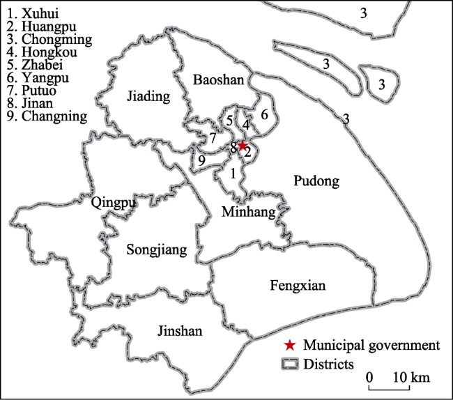
Figure 1 Location of the study area and its administrative structure

3.2 Data sources

The secondary source of urban industrial enterprises is the Shanghai economic census of 2008. It has a total record of 6653 enterprises with the attribute data of company name, address and postcode, composed of clothing garment industry (2680), food processing industry (617), packaging and printing industry (987), interior decoration suppliers (963), cosmetics and washing supplies (230), arts crafts and tourism supplies (717) and small-scale electronics suppliers (459). These enterprises are geo- referenced by using their company names, postal address and basic spatial information from Shanghai Administrative Bureau for Industry and Commerce (Figure 2). Chongming is separated from the main urban area by the Yangtze River and has only a small number of urban industrial enterprises (79), so these areas are excluded for spatial analysis in consideration of the marginal effect (Figure 1). Figure 2 displays the overall spatial distribution of the 6574 urban industrial firms in the main urban area, marked with different colors indicating the type of enterprises. The map clearly displays a marked cluster at the centre of the study area.
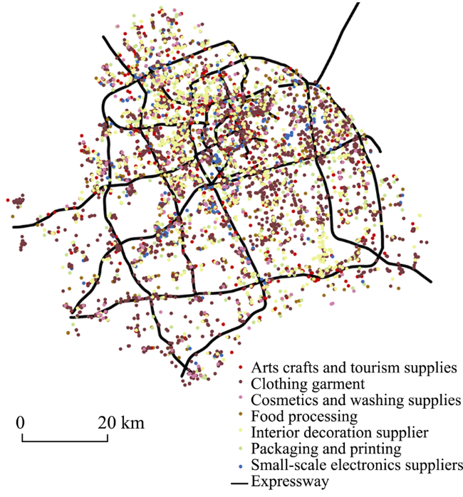
Figure 2 Spatial distribution of all urban industrial firm sites

3.3 Methods

1) Nearest neighborhood analysis (NNA)
In GIS, NNA is a popular method for identifying the spatial pattern of point data - between clustering, random and dispersion distributions. As “first order” statistics, it calculates R statistics comparing the observed average distance between each point and it is the nearest neighbouring point with the expected value. This exact expected average distance is derived using the size of the study area and the total number of points. A value of 1 means a random distribution, 0 a complete clustering and a maximum value for a perfectly uniform distribution. A p-value confirms the statistical significance level of the pattern. NNA provides an overall global interpretation of the spatial distributions but it does not show how the pattern changes with the distance between points and their nearest neighboring points.
2) Kernel density
Kernel density analysis, as a visual tool, is also a popular method for exploring hot spot areas of point data. It uses a moving kernel function to weight points within a search neighborhood by their distance to the location where density is being calculated. The smoothing degree of created surface is dependent on the user-defined bandwidth of the kernel, which reflects the scale of analysis. Such a subjective exploration does not create confirmatory statistics. In summary, NNA and kernel density have overcome the weaknesses of Gini coefficient, Ellison-Glaeser index and location quotient indicator but are not able to solve the multi-scale issue. This study will apply K-function and co-location quotient methods for measuring the spatial concentration of urban industry and particularly examine if there is any co-location between any categories.
3) K-function analysis
Exploring the varying spatial patterns at multiple distances and spatial scales often reflects the particular spatial processes in question. Ripley’s K-function (Ripley, 1976; 1977; 1979), as a spatial distance-based statistical method, provides an estimate and summary of spatial dependence over a wider range of scales. Ripley’s K-function is a second order statistic considering the complete distribution of distances between any pairs of points. It is essentially a cumulative measure, showing the average number of neighbours in an area of circle with radius (r), divided by the density of the whole study region (Equation 1).
$K(r)=\frac{A}{N\times (N-1)}\sum\limits_{i=1}^{N}{\sum\limits_{j=1,i\ne j}^{N}{wijI(dij)}}$ (1)
$I({{d}_{ij}})=\left\{ \begin{align} & 1,\ {{d}_{ij}}\le r \\ & 0,\ {{d}_{ij}}>r\ \\ \end{align} \right.$ (2)
where A is the size of defined study area that might be a rectangular or alternatively a polygon; N is the total number of points; dij is the distance between the ith and jth site; I(dij) is a binary function of dij, either 1 or 0 and wij is a weighting variable to correct for border effects. The edge effect means the sensitivity of the results to the specific area considered. For example, wij will be 1 if the whole circle is completely within the study area, otherwise, measured as proportion of circumference of the circle.
These equations indicate that the K(r) function describes characteristics of the point patterns at many and different scales simultaneously, and illustrates how the spatial clustering or dispersion of point features changes with neighborhood size r. Thereby, K-function is a continuous distance method, rather than a discrete administrative scale method, to measure spatial concentration. As a result, this test is unbiased with respect to scale and aggregation or without the issue of MAUP.
Under the assumption of complete spatial randomness (CSR), the expected number of events within distance r of an event is πr2. If a point pattern is dispersed, then K(r) < πr2; if a point pattern is clustered, then K(r) > πr2. To interpret it, K(r) is transformed into the following L(r):
$L(r)=\sqrt{\frac{K(r)}{\pi }}$ (3)
L function is simply a rescaled K-function. So when L(r) >r, then it is a clustered pattern; if L(r)<r, then a dispersed pattern. In this paper, an unweighted L(r) is selected and calculated by the tool of Multi-Distance Spatial Cluster Analysis (Ripley’s K-function) in ArcGIS 10.2.2. A weighted edge correction method was implemented with a defined polygon boundary data selected. Upper and lower 99% confidence bands were calculated for each L plot using 99 Monte Carlo simulations in the study area boundary.
Using L(r) as y-axis and r as x-axis, Ripley’s K-function graphs, in which solid lines depict the expected value at any distance and dashed lines the observed, enable us to visually evaluate and compare the patterns of these seven industries.
Using the method proposed by Albert et al. (2012), ‘whole of urban industry’ is regarded as a benchmark, the difference in the L(r) function between each sector and the benchmark can be deployed to compare the spatial distribution of each sector with the overall tendency of urban industry to agglomerate:
$Lsb(r)=Ls(r)-Lb(r)$ (4)
where Ls(r), Lb(r) and Lsb(r) are the L(r) values of sector s under consideration, the whole urban industry (benchmark) and the difference between both at distance r. Lsb(r) can be used to measure relative localization or dispersion, which depends on whether Lsb(r)>1 (localization) or Lsb(r) < 1 (dispersion). In both cases, it can be claimed that the sector s is concentrated or dispersed relative to the whole of urban industry. Albert et al. (2012) argued that this method enables us to compare across industry.
4) Co-location quotient
There are several methods to explore co-location in the literature, e.g. bivariate K-function, cross-K-function. Arbia et al. (2008) use the bivariate K-function approach to identify co-location across different industries. However, it measures spatial association between two populations, not the categories in a single population as shown in the study. Leslie and Kronenfeld (2011) proposed a co-location quotient (CLQ) method, aimed to quantify (potentially asymmetrical) spatial association between categories of a population that may itself exhibit spatial autocorrelation. They argued CLQ method provides a measure of the degree to which one categorical subset is spatially dependent on the other in a single population. The co-location of the distribution of two variables is less often studied than is spatial autocorrelation (Cromley et al., 2014). The CLQ method is an extension of location quotient method used by geographers and economists to judge a region’s degree of specialization in a particular industry but it does not have the MAUP issue.
CLQ, measured as a ratio of observed versus expected points of one type among the set of the nearest neighbors of the same or another type in the entire population, particularly recognizes any asymmetric relationships between these categories that may have different sizes of sample (Cromley et al., 2015).
$CLQab=\frac{Cab/Na}{Nb/(N-1)}$ (5)
$Nb=Na-1,\text{ }ifb=a$ (6)
$Cab=\sum\limits_{i=1}^{Na}{\sum\limits_{j=1}^{v}{\frac{Tij}{vi}}}$ (7)
where N is the size of whole industrial population under study, Na and Nb the size of category a and b sample respectively; Cab is the count (or number) of category a points whose nearest neighbor is a category b point. Cab can be represented in Equation 7, in which vi is the number of equidistant nearest neighbors at ith point of category a, and Tij =1 if its jth equidistant nearest neighbor is in category b, otherwise Tij =0.
CLQab denotes the spatial attraction of a to b, or alternatively the degree to which b attracts a. For instance, CLQab = 3 indicates that points of category a are three times as likely to be located near a category b point than would occur randomly.
Like classical location quotients, CLQab > 1 shows a higher number of the nearest neighbors of category b than expected, given the relative counts in its population, whereas CLQab < 1 indicates that points in category b are the closest neighbors to points in category a less frequently than expected. The CLQab value is influenced by both sample sizes and geometric constraints. Its maximum value is calculated as follows:
$Max(CLQab)=Min\left( \frac{N-1}{Nb},\text{ }\frac{5(N-1)}{Na} \right)$ (8)
Asymmetry is defined by the condition that CLQabCLQba including insignificant value.
The global CLQ is defined as the ratio of the observed number of the same category nearest neighbor pairs to that expected number under the null hypothesis of no spatial association between categories.
$CLQglobal=\frac{\sum\limits_{X=1}^{N}{Cxx}}{\sum\limits_{X=1}^{N}{Nx\times \left( \frac{Nx-1}{N-1} \right)}}$ (9)
where x is one category of the population, Nx is the size of the X sample, Cxx is the CLQ value of x category to itself. The statistical significance in Equations 3 and 9 is derived using randomized Monte Carlo simulations. The CLQ can be viewed as a simple modification of either the join count statistic or the cross-K-function (Leslie and Kronenfeld, 2011).

4 Results and analysis

The analysis methods mentioned above are implemented with ArcGIS 10.2.2 and CLQ (http://seg.gmu.edu/#page1). These results and maps enable us to identify and explain the clustering and co-location patterns.

4.1 The spatial distribution of urban industry

To compare the spatial distributions between the seven categories, a same kernel (5 km neighbourhood) and function is applied for the Kernel density analysis of each category, the created surfaces are presented in Figure 3, in which similarity, and disparity in concentration can be detected.
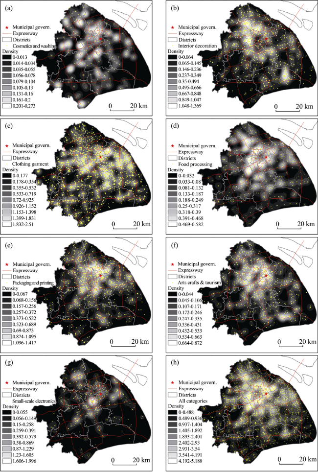
Figure 3 Kernel density of (a) Cosmetics and washing; (b) Interior decoration; (c) Clothing garment; (d) Food processing; (e) Packaging and printing; (f) Arts crafts and tourism; (g) Small-scale electronics; (h) All categories
First, not only city centre, but also the urban fringe accommodates the highest concentration of different category firms though their numbers of firms are varied. Large-size concentric agglomerations are formatted to surround the inner city or city centre, which is different from the location pattern of traditional industry (Gaubatz, 1999) in the process of suburbanization. Second, different category firms demonstrate a distinct pattern, all of which can be classified into three models: homogeneous, centric, and location specific clustering. The first model includes cosmetics and washing and clothing garment. Particularly the latter demonstrates a pattern of clustering at a small scale, but dispersion at a large scale. The second model comprises of food processing, packaging and printing, and arts crafts and tourism, with a clear tendency to city centre and urban fringe. The third model is for small-scale electronics, which has two clusters in the central and north respectively, with a specific preference to some areas.
Third, these concentrations are mostly located in industrial parks (in the city centre) or development zones (in the urban fringe). The well-known development zones include Hongqiao Economic Development Zone, Caohejing High-tech Development Zone, Zhangjiang Hi-tech Development Zone, Jinqiao Development Zone and Waigaoqiao Free Trade Zone, which are administered at three levels: national, municipal and county. The development zone at different levels has specific requirements for its site selection and the firms to be located there, which influence the spatial distribution of urban industrial firms across the study area. High-tech firms are mostly concentrated in national development zone. The firms located in municipal or county-level zone are highly diverse. For example, the concentration of packaging and printing industry is seen in Shanghai Printing and Media Industrial Park (in Zhabei District) and Shanghai International Centre for Packaging and Printing (in Putuo District). The concentration of clothing garment industry is witnessed in Shanghai Printing and Media Industrial Park (in Zhabei District) and Shanghai International Industrial Park for Family Textile (in Yangpu District) and Hongqiao Industrial Park of High-quality Clothing Garment (in Hongqiao District). In a sum, different categories have distinguished spatial patterns.
To further visualize the relative distribution to the city centre (the site of Municipal Government or People’s Square), the total number of each category firms within each 1-km buffer zone is summarized and presented in a graph (Figure 4), from which the influence of urban morphology on their distributions can be detected. All categories share a very similar non-linear trend, with an increasing intensity up to the peak distance (between 21-30 km) and then decreasing away until about 50 km. It means urban fringe areas are attractive than city centre and rural area for some categories.
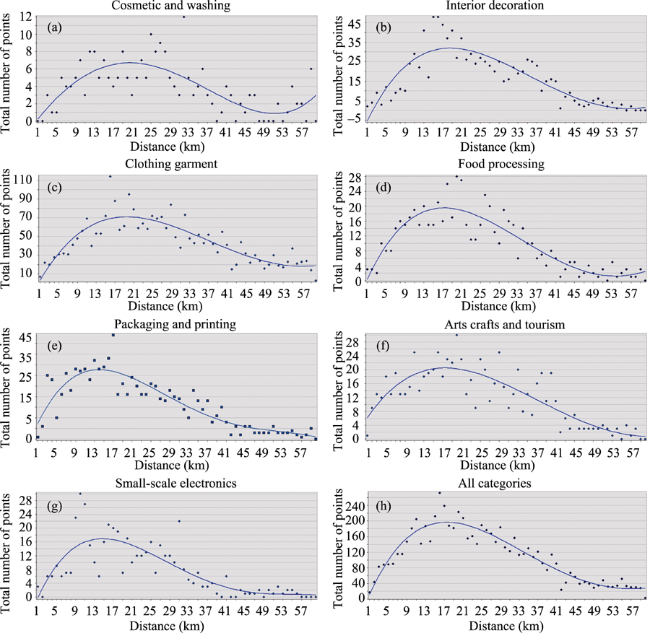
Figure 4 Relative distribution to the city centre from (a) Cosmetics and washing; (b) Interior decoration; (c) Clothing garment; (d) Food processing; (e) Packaging and printing; (f) Arts crafts and tourism; (g) Small-scale electronics; (h) All categories
This pattern might be contributed from differential rent, the changing local policy of economic development (the shift of focus from on the secondary industry to on the tertiary industry). The increasing land price in the city centre has driven the relocation of these firms away. The local policy of industrial restructuring (secondary out and tertiary in) has reduced the number of firms in city centre. Conversely, the preferential policies based on both its tax and employment demand made by each district government, which led to the reduction of rent for these firms, and the better access to transport infrastructure and facilities in the urban fringe have made the buffering zone around 21-30 km from city centre the most suitable locations for urban industrial firms.
Two categories: packaging and printing and arts crafts and tourism have a relatively higher intensity in the city centre than the rest in Figure 4. The statistical comparisons between the seven categories are also summarized into Table 1.
Table 1 Comparisons between categories in relative distribution to the city centre
Type Peak value Value at 100 km Distance (km) Decreasing rate
All categories 1.29 0.628 27 0.0091 (7)
Cosmetics and washing 1.3 0.642 29 0.0093 (6)
Interior decoration 1.34 0.619 24 0.0095 (4)
Clothing garment 1.24 0.645 30 0.0085 (8)
Food processing 1.34 0.616 28 0.01 (2)
Packaging and printing 1.39 0.61 21 0.0099 (3)
Arts crafts and tourism 1.33 0.614 24 0.0094 (5)
Small-scale electronics 1.42 0.59 27 0.011 (1)
Table 2 presents the results of NNA, in which all categories show statistically significant pattern of clustering (as ratio << 1 and z-score < -8). By contrast, the clothing garment is most clustered with an average nearest distance of 403 meter, followed closely by entire industry; and cosmetics and washing is the least with about 2 km average nearest distance, and with all the rest having similar values of average nearest distance. Thereby, cosmetics and washing has the largest separation space between each firm and its nearest competitor but clothing garment has the shortest. Both categories are closely linked with daily lives of residents but relatively the shortest spatial separation of clothing garment is contributed by small-scale employment in each firm and a large quantity of its firms across the study area, the largest distance interval of cosmetics and washing by a small quantity of firms in total.
Table 2 Results of the nearest neighborhood analysis
Type 1 2 3 4 5 6 7 All
Observed distance 1130 828 947 972 403 816 1997 231
Expected distance 2022 1520 1771 1918 963 1420 2857 519
Ratio 0.559 0.545 0.535 0.507 0.418 0.575 0.70 0.444
Z-score -20.9 -27.36 -23.83 -20.22 -57.62 -25.25 -8.7 -86.23
Sample size 599 984 710 456 2643 958 224 6574

1. Food processing; 2. Packaging and printing; 3. Arts crafts and tourism; 4. Small-scale electronics; 5. Clothing garment; 6. Interior decoration; 7. Cosmetics and washing

4.2 K-function

K-function method is applied for two analyses: each category (Equation 3) and comparison between each category and the whole urban industry (Equation 4), which are represented in Figures 5 and 6 respectively.
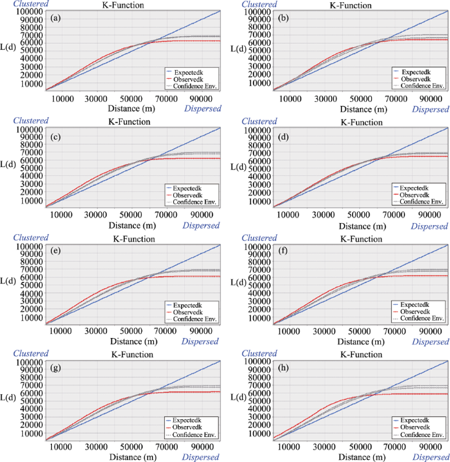
Figure 5 K-functions of (a) All; (b) Cosmetics and washing; (c) Interior decoration; (d) Clothing garment; (d) Food processing; (f) Packaging and printing; (g) Arts crafts and tourism; (h) Small-scale electronics
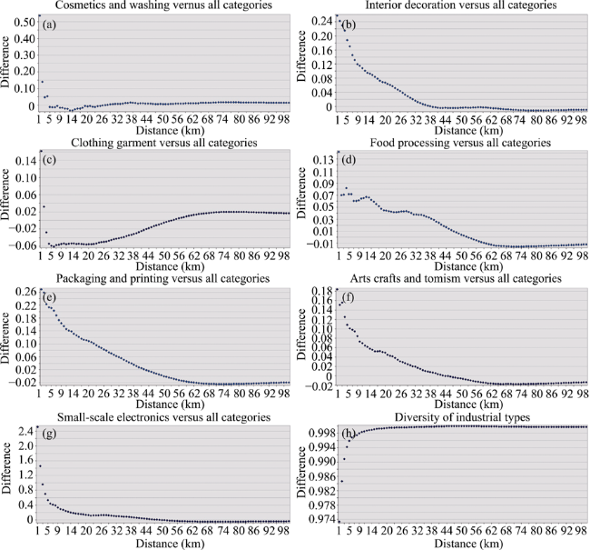
Figure 6 Comparisons with the benchmark (a) Cosmetics and washing; (b) Interior decoration; (c) Clothing garment; (d) Food processing; (e) Packaging and printing; (f) Arts crafts and tourism; (g) Small-scale electronics; (h) Diversity
The graphs reported in Figure 5 display the behavior of the functions L(d) at the various distances d for the seven categories of the urban industry and the whole. The confidence envelopes shown in the graphs referred to the null hypothesis at a significance level α=0.01. The value d corresponding to the peaks of the observed line outside the confidence envelopes represents the distance at which there is significant spatial concentration. A quick look at the results shown in Figure 5 reveals a weak phenomenon of spatial concentration at shorter distances - less than 10 km - then increasing concentration from 10 up to 50 km for all the sectors of the urban industry. The maximum value is achieved at about 30 km for nearly all sectors.
To compare the patterns between the seven sectors, the whole urban industry is selected as a benchmark or reference point, the difference of L(d) functional values between each category and the benchmark is illustrated in Figure 6, in which the disparity between sectors can be much easily detected than in Figure 5. These graphs enable us to identify the distance ranges of significant concentrations and dispersions and their separate peak values and distances, which are summarized in Table 3. Three typical patterns can be identified from Figure 6.
Table 3 Location pattern of each category in relation to the whole urban industry
Category Significant concentration Significant dispersion Peak value Peak distance
Cosmetics and washing 0-4 km - 0.55 1 km
Interior decoration 0-37 km - 0.26 1 km
Clothing garment 0-1 & 54-100 km 1-54 km 0.16 & 0.02
-0.06
1 km, 70 km
6 km
Food processing 0-54 km 54-100 km 0.14
-0.02
1 km
70 km
Packaging and printing 0-50 km 54-100 km 0.27
-0.02
1 km
70 km
Arts crafts and tourism 0-43 km 43-100 km 0.185
-0.02
1 km
66 km
Small-scale electronics 0-44 km - 2.5 1 km
First, cosmetics and washing is more randomly distributed with a low degree of clustering due to its relatively homogeneous distribution across the study area. Second, the five categories (Interior decoration, Food processing, Packaging and printing, Arts crafts and tourism and Small-scale electronics) share a similar pattern: gradual transformation from clustering at short distance into random at longer distance because most of these firms are located in city centre and urban fringe. Third, clothing garment is random at short distance and more clustered at longer distance, reflecting the relocation of this sector from the city centre to urban fringe. The 8th graph in Figure 6 shows the entropy-based diversity is very high throughout all the distance ranges and reaches its maximum value 100% very quickly around 20 km, compared with the complex pattern of spatial concentration.
In Table 3, first, none are clustered or dispersed across all distances when 100 km is set as the distance limit within the study area in the graphs. Second, all categories share the loca- tional concentration within 1 km distance with varied degree of clustering, being the highest in small-scale electronics and the lowest in food processing. Third, cosmetics and washing shows clustering only at short distance (less than 4 km) and then turn to random. By contrast, interior decoration and small-scale electronics share the same trend but extend the distance range of concentration from 4 km to 37 km and 44 km respectively. Fourth, clothing garment is the only one category showing a dispersed pattern (1-54 km) between two clustering patterns (less than 1 km and more than 54 km). Fifth, food processing, packaging and printing and arts crafts and tourism share similar pattern apart from slightly different values in peak values and distances. Finally, it is evidential that the degree of concentration is much higher than that of dispersion.

4.3 Co-location analysis

Co-location quotient analysis is applied for two cases: pairs between seven categories, pairs between regrouped productive (Clothing garment, Cosmetics and washing, Food processing) and consumptive (Arts crafts and tourism, Interior decoration; Packaging and printing; Small-scale electronics). The CLQ analysis was implemented 9999 times to achieve a significance level of 1%. After removing those insignificant results, the CLQ results are represented in Table 4.
Table 4 Co-location quotient results
Category 1 2 3 4 5 6 7
1 1.247 1.116 ** 0.95
2 1.285 1.066** 0.914 0.923
3 1.052** 1.339 0.858 0.913
4 0.779 3.56 0.715 0.771
5 0.877 0.859 0.888 0.71 1.224 0.835
6 0.937** 1.059* 0.819 0.89 1.421
7 0.943** 1.906
Sample 710 2643 224 599 958 984 456

1. Arts crafts and tourism; 2. Clothing garment; 3. Cosmetics and washing; 4. Food processing; 5. Interior decoration; 6. Packaging and printing; 7. Small-scale electronics

**: 0.05 level; *: 0.1 level; No note: 0.01 level

The global CLQ (1.385, calculated according to Equations 5 and 9) is very positive but a weak tendency of co-location globally. The pairwise CLQs shown in Table 4 reveal four types of disaggregate information. First, significant-type autocorrelation is strong as all p-values are close to 0.
The same-category pairwise CLQs (diagonal) that are significant and greater than 1, indicates that industries of all seven categories have strong preferences for co-locating with other industries of the same category. It means all seven types of industry are more likely to have neighbors of the same category than indicated by a random distribution, or rather, each demonstrates a clustering pattern. However, there is a large variation in the degree of autocorrelation between the seven categories, with the following orders: food processing (3.56); small-scale electronics (1.906); packaging and printing (1.42); clothing garment (1.285); cosmetics and washing (1.339); arts crafts and tourism (1.247); and interior decoration (1.224). This variation contributes to the low value of global CLQ (1.385). The strongest effect is present in food processing, which is more than three times as likely to have another food-processing firm as its nearest neighbor. Food processing firms are usually very close to both users (local residents) and materials (markets), and very sensitive to its production environment, resulting in massive clustering in specific areas (e.g. large residential areas). This effect is the weakest for interior decoration, which is just 1.224 times more likely to have another industry of the same category as their nearest neighbor. Interior decoration firms occupy a larger area, have weak technical linkage with others and produce noise pollution, leading to its low degree of clustering.
Second, the significant two-way associations: CLQ (1→5) =0.95 and CLQ (5→1) = 0.877 indicate both the industry of arts crafts and tourism and the industry of interior décoration exclude (or separate) from each other as each avoids to collocate with another (CLQ is less than 1). Nearly same level of exclusion also applies to the following symmetrical associations: clothing garment / interior decoration (0.914 versus 0.859), clothing garment / packaging and printing (0.923 versus 0.937), cosmetics and washing / food processing (0.858 versus 0.778), cosmetics and washing / interior decoration (0.913 versus 0.888), food processing/interior decoration (0.715 versus 0.71), food processing/ packaging and printing (0.771 versus 0.819), and interior decoration/packaging and printing (0.835 against 0.89). It can be concluded from these analyses that interior decoration is excluded by all the six categories and the three categories (cosmetics and washing, food processing, interior décoration) exclude with each other. The former result suggests weak technical linkages and the varied environment of production between them, whilst the latter mainly explained by the exclusive environment of production between them.
Third, the significant two-way associations CLQ (2→3) =1.066 and CLQ (3→2) = 1.052 indicate both the industry of clothing garment and the industry of cosmetics and washing co-locate with each other as each prefers or co-locates with another (CLQ is slightly larger than 1). Both have mutual spatial attraction though this association is not very strong (at 5% significance level). Such co-location pattern indicates there might be a chain of industry between both because the materials of clothing garment including fiber, leather, waterproof and perfume are manufactured by cosmetics and washing firms.
Fourth, there are two asymmetrical associations. Food processing is attractive to arts crafts and tourism (or the latter is dependent on the former) but not vice versa (CLQ (1→4) =1.116 but CLQ (4→1) not significant). Cosmetics and washing only attractive to packaging and printing (or packaging and printing is dependent on cosmetics and washing) (CLQ (6→3) =1.059* but CLQ (3→6) not significant). Many products from food processing may be on market for arts crafts and tourism. Likely, products from cosmetics and washing firms need to be packaged and advertised massively using packaging and printing materials.
Fifthly, the newly classified two categories (productive and consumptive) have very similar values in auto-correlation (1.114 against 1.107, but all >1) and co-location (0.873 against 0.904, but all <1). It means each group clusters by itself and is independent of another.

5 Discussion and conclusions

5.1 Conclusions

In this study, K-function and CLQ methods have demonstrated remarkable capabilities of analyzing locational and co-location patterns as both methods are distance-based measures without MAUP issue caused by discrete spatial units. Compared with NNA and kernel density analysis, K-function and its extended Lsb function are able to not only statistically confirm the spatial pattern (clustered or dispersed) but also visually detect the changes of spatial patterns with distance and corresponding peak values/distances. The CLQ method, focusing on spatial dependence between categories in a same population, enables to distinguish two-way dependence. All these methods provide more complementary details and insights into the patterns under study. All these advantages benefit from the use of micro-level point data in 2008, based on which this study has found the following facts.
First, the city centre and the urban fringe have the highest intensity of urban industrial firms, but the zones with 20-30 km from the city centre is a watershed for most categories. The intensity of these firms decreases with distance after the watershed distance, with the small-scale electronics being the fastest and the clothing garment being the slowest.
Second, each category demonstrates a varied degree of spatial concentration, with clothing garment being the highest, cosmetics and washing being the lowest. The degree of concentration varies with distance, weaker at shorter distance, increasing up to the maximum distance of 30 km and then decreasing until 50 km.
Third, compared with the entire urban industry, there are several types of patterns: mixture of clustered, random and dispersed distribution at a varied range of distances. Small-scale electronics is most clustered and food processing the least. Cosmetics and washing is only clustered within 4 km. Clothing garment is the only one showing a dispersed pattern at the large range of distance (1-54 km).
Fourth, food processing is most likely to have another same category firm as its nearest neighbor, contrasting with the least likely one-interior decoration. Only clothing garment, cosmetics and washing prefer to co-locate with each other as a consequence of comparison shopping and functional complementarity. Food processing is attractive to arts crafts and tourism, cosmetics, and washing only attractive to packaging and printing, but not vice versa. Particularly, interior decoration is less preferred by all the six categories and the three categories (Cosmetics and washing, Food processing, and Interior decoration) locate far away from each other.

5.2 Discussion

The occurrence of urban industry results from the joint forces of multiple factors - politics, society, economy and environment at several levels (Figure 7), which underpin either push or pull forces. Industrial decentralization from urban cores is one of the forces driving the restructuring in Chinese cities (Qian, 2012). Compared with traditional industry, however, urban industry is part of a modern industrial system characterized by high-level accessibility of employment, high adaptability to change, low environmental pollution, high taxation, and fast-added values. This context enables businesses that might otherwise have to disperse to lower cost sites, to remain in-situ within central and competitive business areas in China.
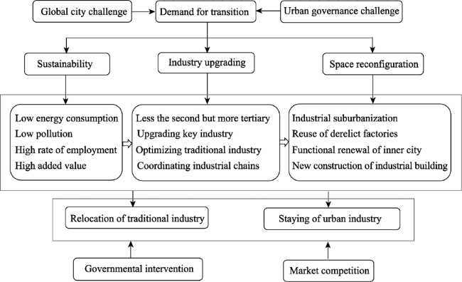
Figure 7 A conceptual framework of the emergence and layout of urban industry in Shanghai
Many challenges and conflicts accompany attempts to upgrade cities from local and regional centres to global cities. A global city will require a high-level urban functional system and optimal spatial configuration. Environmental pollution and traffic jams prevailing in mega cities also demand effective and efficient urban governance. Consequently, this has increased pressure to reform or re-orientate local government within China to enable cities to become more competitive (Qian, 2012).
Successful urban transformation should also meet the objectives of sustainable development, through industrial upgrading and optimal spatial configuration. Industrial upgrading is defined as the process by which economic actors: nations, firms, and workers, move from low-value to relatively high-value activities in global production networks (Gereffi, 2009). First, only the firms that consume less energy, produce less pollution, provide local people with more job opportunities, and generate more tax income are able to remain in the central city. Second, to achieve this level of sustainability, the traditional industries must be upgraded, to promote sectoral shift from secondary industry to tertiary activity, and through coordination of relevant industrial supply-chains. Third, during the process of industrial upgrading, those firms failing to sustainability targets, will be relocated out of the city-centre or even forced to exit the market. Vacated industrial buildings might be reused for other functions to promote urban regeneration. Those firms meeting the designated objectives will remain in-situ to comprise an urban industrial sector. The processes driving urban industrial formation, therefore, encompass market competition based on rent bid and utility maximization principles, as well as governmental intervention through planning, finance and tax policies. This combination shaped the unique patterns of urban industry, such as agglomeration and clustering at specific locations (Yang et al., 2015).
For example, the Buyecheng industrial park (Figure 8), located on 610 Henfeng Road in Zhabei District was transformed or renewed from an original Huafeng China Factory into a modern industrial park by Shanghai Urban Industry Development Cooperation. The area of the park is 5972 m2, with 18,000 m2 floor space. The renewal of this factory has benefited from the cheap land resource, unused factory space, complete facility provision, good access to transport at the site, and preferential local policies. With strategically reasonable design and management, this site has developed into the industrial park with enjoyable environment, good accessibility, and mixed functionalities of product development, manufacturing, and marketing.
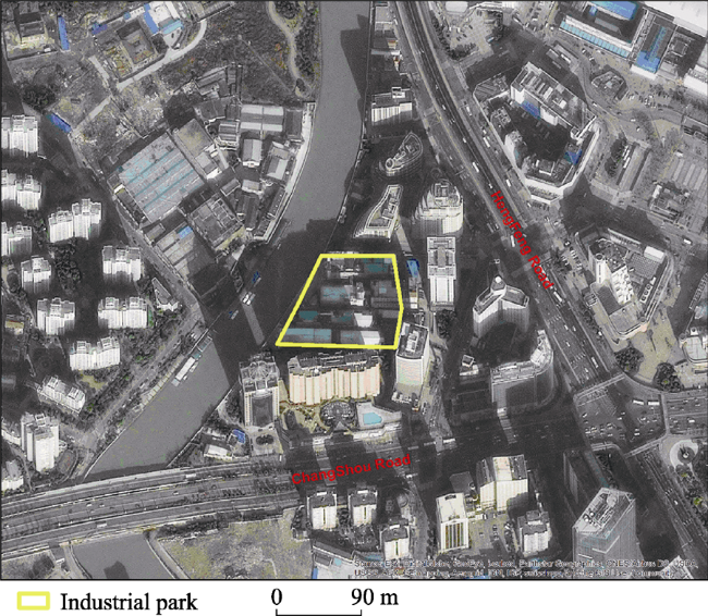
Figure 8 An example of industrial park - Buyecheng industrial park
Consequently, the different pattern of each category indicates that economic sectors benefit differently from spatial clusters. The patterns revealed in this study exhibit that the amount of concentration cannot be explained by factors such as rent, transportation facilities, environmental limits and labour employment. Colocating firms benefit from access to shared resources like infrastructure, and a local, specialized labour market (Voinea and Van Kranenburg, 2011).
The location pattern of urban industry appears to contrast to traditional industry and is determined by multiple factors. First, the firm must meet the surviving conditions including light or no pollution, low energy consumption, high added-value, and high opportunity of employment. Second, it is largely affected by the inertia of urban development history and embeddedness of industrial development. During the process of economic transition, the force of inertia means that certain firms will remain at the intermediate stage. The force of embeddedness, including technical linkages between firms and market demand and supply, also facilitate the survival of these firms. A third factor is policy. Each district government has supporting policies that reflect various perspectives, including financial revenue, rate of employment and influence of creative and industrial design. A fourth factor includes differential rent and locational influence. The high land price in the city centre forces industrial firms to move out, but preferential policies might distort the rent curve. In addition, a high level of transport accessibility and proximity to city centre might promote the urban fringe as the best sites for their location. This combination has shaped the unique patterns of urban industry, such as agglomeration and clustering at specific locations (Yang et al., 2015).
Gaubatz (1999) compared the changes in industrial location in the 1980s between Beijing, Shanghai and Guangzhou and found Shanghai retained a high level of industrial development within the city centre as still 48% of industries were located in city districts in 1992, contrasted with 16% and 27% located in central cities of Beijing and Guangzhou in 1989 respectively. It means the current location pattern of urban industry in Shanghai is significantly affected by development inertia. Comparatively, Beijing has adopted another strategy - relocating industrial firms to rural areas (Gao et al., 2014). This implies that unban-industry might be only an intermediate outcome of urban industrial restructuring as industrial suburbanization (Qian, 2012) might be its final outcome for Shanghai the same as Beijing and what happened in the Western world.
Urban industry, however, might be replaced by tertiary activity (or 2.5 industry between secondary and tertiary) or by differential rent. In general, the presence of urban industry is positive for sustainable urban development, providing job opportunities, tax and coordinated economic services in the city centre during the process of economic transition. Accordingly, all these would enable to mitigate the negative influences of urban hollowness and provide support for the preservation of urban heritages at the current stage, industrial suburbanization may cause decentralization of employment opportunities and this will further extend the commuting distance of employees who prefer to stay in city centre for better social, economic and cultural activities. Relocation of firms to outer rural area also causes great damage to the ecological environment, results in the shrinkage in urban manufacturing industry, and directly brings sluggish growth in service industry and poses pressure on urban employment.
In the future, more comparative case studies might answer whether Western agglomeration theories can explain the industrial restructuring in contemporary urbanization in China. They might also reveal how industrialisation is also affected by the legacies of contemporary state policies (Liu, 2014). The current methodology is subject to the following two deficiencies: lack of attribute (e.g. employees in each firm) and temporal (e.g. registration year of these urban industrial firms in the past decades) data; a global rather than a local analysis method. With spatio-temporal data, the process instead of only pattern of industrial restructuring can be explained. Using local analysis method, such as geographically weighted co-location quotient (Cromley et al., 2014), not only spatial dependence but also spatial heterogeneity or more specifically spatial non-stationarity can be incorporated into the statistical analysis.

The authors have declared that no competing interests exist.

[1]
Albert J M, Casanova M R, Orts V, 2012. Spatial location patterns of Spanish manufacturing firms. Papers in Regional Science, 91(1): 107-136 .

[2]
Arbia G, Espa G, Quah D, 2008. A class of spatial econometric methods in the empirical analysis of clusters of firms in the space. Empirical Economics, 34: 81-103 .

[3]
Bai C E, Du Y, Tao Z et al., 2004. Local protectionism and regional specialization: Evidence from China’s industries. Journal of International Economics, 63: 397-417 .

[4]
Behrens K, Bougna T, 2015. An anatomy of the geographical concentration of Canadian manufacturing industries. Regional Science and Urban Economics, 51: 47-69 .

[5]
Chen S, Jefferson G H, Zhang J, 2011. Structural change, productivity growth and industrial transformation in China. China Economic Review, 22(1): 133-150 .

[6]
Cheng F, van Oort F, Geertman Set al., 2014. Science parks and the co-location of high-tech small- and medium- sized firms in China’s Shenzhen.Urban Studies, 51(5): 1073-1089 .

[7]
Cromley E K, Wilson-Genderson M, Christman Z et al., 2015. Colocation of older adults with successful aging based on objective and subjective measures. Applied Geography, 56: 13-20 .

[8]
Cromley R G, Hanink D M, Bentley G C, 2014. Geographically weighted colocation quotients: Specification and application. The Professional Geographer, 66(1): 138-148 .

[9]
Ellison G, Glaeser E, 1997. Geographic concentration in U.S. manufacturing industries: A dartboard approach. Journal of Political Economy, 105: 889-927 .

[10]
Fang Chuanglin, Liu Xiaoli, 2009. Temporal and spatial differences and imbalance of China’s urbanization development during 1950-2006. Journal of Geographical Sciences, 19(6): 719-732 .

[11]
Fujita M, Krugman P R, Venables A J, 2004. The spatial economy: Cities, regions, and international trade. Am. J. Agric. Econ., 86(1): 283-285.

[12]
Gao Boyang, Liu Weidong, Michael Dunford, 2014. State land policy, land markets and geographies of manufacturing: The case of Beijing, China. Land Use Policy, 36: 1-12 .2013.06.007

[13]
Gaubatz P, 1999. China’s urban transformation: Patterns and processes of morphological changes in Beijing, Shanghai and Guangzhou. Urban Studies, 36(9): 1495-1521 .

[14]
He C, Wang J, 2012. Regional and sectoral differences in the spatial restructuring of Chinese manufacturing industries during the post-WTO period. GeoJournal, 77(3): 361-381 .

[15]
He C, Wei Y D, Xie X, 2008. Globalization, institutional change, and industrial location: Economic transition and industrial concentration in China. Regional Studies, 42(7): 923-945 .

[16]
Hu C, Xu Z, Yashiro N, 2015. Agglomeration and productivity in China: Firm level evidence. China Economic Review, 33: 50-66 .

[17]
Koster H R A, van Ommeren J, Rietveld P, 2014. Estimation of semiparametric sorting models: Explaining geographical concentration of business services. Regional Science and Urban Economics, 44: 14-28 .

[18]
Krugman P, 1991a. Geography and Trade. Cambridge, MA: MIT Press.

[19]
Krugman P, 1991b. Increasing returns and economic geography. Journal of Political Economy, 99: 483-499 .

[20]
Leslie T F, Frankenfeld C L, Makara M A, 2012. The spatial food environment of the DC metropolitan area: Clustering, co-location, and categorical differentiation.Applied Geography, 35(1/2): 300-307.The objective was to analyze the spatial food environment of the Washington, DC metropolitan area. Poorer food sources (convenience stores, fast food, and pharmacies) were the most spatially clustered. Co-Location results suggest strong positive autocorrelation among food environment establishment categories, and competitive effects between pharmacies and convenience stores. Grocery stores were present throughout the region. Changes in the retail food environment, a measure potentially important for diet-related health, occurred through the changing ratio of restaurants to fast food as well as the increased presence of convenience stores.

DOI

[21]
Leslie T F, Kronenfeld B J, 2011. The colocation quotient: A new measure of spatial association between categorical subsets of points. Geographical Analysis, 43(3): 306-326 .

[22]
Liu Z, 2014. Global and local: Measuring geographical concentration of China’s manufacturing industries. The Professional Geographer, 66(2): 284-297 .

[23]
Lu J, Tao Z, 2009. Trends and determinants of China’s industrial agglomeration. Journal of Urban Economics, 65(2): 167-180 .

[24]
Ma Li, Jin Fengjun, Song Zhouying et al., 2013. Spatial coupling analysis of regional economic development and environmental pollution in China. Journal of Geographical Sciences, 23(3): 525-537 .

[25]
Marshall A, 1890. Principles of Economics. London: MacMillan.

[26]
Pan F, Xia Y, 2013. Location and agglomeration of headquarters of publicly listed firms within China’s urban system.Geographical Research, 35(5): 757-779.Headquarters of large firms are the commanding centers of the economy.It is of particular interests to investigate the headquarters' distribution in China,a fast growing transition economy.However,little attention has been paid to the understanding of spatial pattern of headquarters of public companies,which dominates China's economy today.Using a comprehensive dataset of Chinese public listed firms,this paper seeks to find out the spatial pattern of public companies' headquarters and its evolution over time.First,headquarters of public listed firms are mostly located in the eastern China,especially in the Yangtze River Delta,Pearl River Delta and Beijing-Tianjin region.Second,headquarters of the public companies are inclined to be proximate to political centers at different geographical scales.Beijing,as the capital of China,houses most of the headquarters of public firms,and the provincial capital city usually accommodates the largest number of headquarters within its province.Third,Beijing,Shanghai and Shenzhen are the top three cities in terms of the number of public companies' headquarters as well as the scale of the firms.The three cities dominate the first three positions in almost all sectors in terms of the number of headquarters.As the capital of China,Beijing dominates and outperforms other cities.Fourth,headquarters of large firms in China are less agglomerated compared to those much developed countries and are becoming more agglomerated in the cities in coastal China.The number of headquarters in Beijing,Shanghai and Shenzhen is increasing faster compared with other smaller cities.Finally,the number of headquarters is highly correlated with the development of financial industry,airport volume,economic output,globalization,total population,and political level of the city

DOI

[27]
Qian Z, 2012. Post-reform urban restructuring in China: The case of Hangzhou 1990-2010. Town Planning Review, 83(4):431-455 .

[28]
Ripley B D, 1976. The second-order analysis of stationary point processes.Journal of Applied Probability, 13(2): 255-266.This paper provides a rigorous foundation for the second-order analysis of stationary point processes on general spaces. It illuminates the results of Bartlett on spatial point processes, and covers the point processes of stochastic geometry, including the line and hyperplane processes of Davidson and Krickeberg. The main tool is the decomposition of moment measures pioneered by Krickeberg and Vere-Jones. Finally some practical aspects of the analysis of point processes are discussed.

DOI

[29]
Ripley B D, 1977. Modelling spatial patterns. Journal of the Royal Statistical Society - Series B (Methodological), 39: 172-192.

[30]
Ripley B D, 1979. Test of ‘randomness’ for spatial point patterns. Journal of the Royal Statistical Society - Series B (Methodological), 41: 368-374.

[31]
Shanghai Municipal Statistics Bureau (SMSB), 2009. Shanghai Statistical Yearbook (2008). Beijing: China Statistics Press China Statistics Press.

[32]
Shanghai Municipal Statistics Bureau (SMSB), 2011. Shanghai Statistical Yearbook (2010). Beijing: China Statistics Press. .

[33]
Südekum J, 2006. Concentration and specialisation trends in Germany since Reunification. Regional Studies, 40(8): 861-873 .

[34]
Tobler W R, 1970. A computer movie simulating urban growth in the Detroit Region.Economic Geography, 46: 234-240.

DOI

[35]
Voinea C L, Van Kranenburg H, 2011. Colocation patterns of foreign-owned firms in a small open economy: Evidence from the Netherlands. European Planning Studies, 19(12): 2047-2072 .

[36]
Wen M, 2004. Relocation and agglomeration of Chinese industry. Journal of Development Economics, 73(1): 329-347 .

[37]
Xi H, Cai Y, 2013. Discussion on urban industrial space organizations and the formation mechanism of Shanghai.E-Journal of China Urban Studies, 8(2): 102-109. (in Chinese)

[38]
Yang C, 2012. Restructuring the export-oriented industrialization in the Pearl River Delta, China: Institutional evolution and emerging tension. Applied Geography, 32(1): 143-157 .

[39]
Yang Z, Hao P, Cai J, 2015. Economic clusters: A bridge between economic and spatial policies in the case of Beijing. Cities, 42(Part B): 171-185 .

[40]
Yuan F, Wei Y D, Chen W, 2014. Economic transition, industrial location and corporate networks: Remaking the Sunan Model in Wuxi City, China. Habitat International, 42: 58-68. 2013.10.008.

Outlines

/