Research Articles

Automatic mapping of lunar landforms using DEM-derived geomorphometric parameters

  • WANG Jiao , 1, 2 ,
  • CHENG Weiming , 2, * ,
  • ZHOU Chenghu 2 ,
  • ZHENG Xinqi 1
Expand
  • 1. School of Information Engineering, China University of Geosciences, Beijing 100083, China
  • 2. State Key Laboratory of Resources and Environmental Information System, Institute of Geographic Sciences and Natural Resources Research, CAS, Beijing 100101, China
*Corresponding author: Cheng Weiming (1973-), Professor, E-mail:

Author: Wang Jiao (1990-), PhD, specialized in planetary geomorphology and spatial analysis. E-mail:

Received date: 2017-06-13

  Accepted date: 2017-07-31

  Online published: 2017-09-07

Supported by

National Natural Science Foundation of China, No.41571388

National Special Basic Research Fund, No.2015FY210500

Copyright

Journal of Geographical Sciences, All Rights Reserved

Abstract

Developing approaches to automate the analysis of the massive amounts of data sent back from the Moon will generate significant benefits for the field of lunar geomorphology. In this paper, we outline an automated method for mapping lunar landforms that is based on digital terrain analysis. An iterative self-organizing (ISO) cluster unsupervised classification enables the automatic mapping of landforms via a series of input raster bands that utilize six geomorphometric parameters. These parameters divide landforms into a number of spatially extended, topographically homogeneous segments that exhibit similar terrain attributes and neighborhood properties. To illustrate the applicability of our approach, we apply it to three representative test sites on the Moon, automatically presenting our results as a thematic landform map. We also quantitatively evaluated this approach using a series of confusion matrices, achieving overall accuracies as high as 83.34% and Kappa coefficients (K) as high as 0.77. An immediate version of our algorithm can also be applied for automatically mapping large-scale lunar landforms and for the quantitative comparison of lunar surface morphologies.

Cite this article

WANG Jiao , CHENG Weiming , ZHOU Chenghu , ZHENG Xinqi . Automatic mapping of lunar landforms using DEM-derived geomorphometric parameters[J]. Journal of Geographical Sciences, 2017 , 27(11) : 1413 -1427 . DOI: 10.1007/s11442-017-1443-z

1 Introduction

Landforms are the result of geologic and geomorphologic processes that occur on the surface of the Earth and other planets (Bolongaro-Crevenna et al., 2005). Accurately collecting and processing information about landforms is necessary for landscape evaluation, hazard prediction, suitability and erosion studies, as well as various landscape and regional planning (Drăguţ and Blaschke, 2006). Consequently, mapping landforms on the surfaces of planets at broad spatial scales is becoming increasingly important; easily accessible digital elevation model (DEM) data has led to the development of a growing number of automated landform mapping techniques that utilize remote sensing (RS) and geographic information system (GIS) approaches (Butle and Walsh, 1998; Florinsky, 1998; Ehlers et al., 2002).
One pixel in a DEM encapsulates an elevation value vector as well as other extractable measures that relate to basic components of terrain, including slope, aspect, convexity, and relief amplitude. It is also expected to be the case that pixels constituting a particular landform will encapsulate similar terrain vectors; these vectors are considered to be similar if the Euclidean distance between them is small (Giles and Franklin, 1998; Miliaresis, 2001; Bue and Stepinski, 2006). Thus, landform classification can be achieved by applying a clustering algorithm across all attribute vectors to determine their exclusive similarity at a given site. Enabling these comparisons is the true value of a DEM and the essence of the classification method.
A range of manual methods was used in the past to classify macro-morphologic landforms from contour maps or stereo aerial photographs. However, as these approaches are relatively time-consuming and generate results that depend on subjective decisions made by the interpreter, they are less suitable for the efficient analysis of large datasets. Thus, a series of automated methods has been developed to identify individual terrain features; physical characteristics can be extracted from a DEM using a variety of methods including the combination of morphometric parameters like slope gradient, local convexity, and surface texture (Iwahashi and Pike, 2007), as well as fuzzy logic and unsupervised classification (Burrough et al., 2000; Adediran et al., 2004), supervised classification (Hengl and Rossiter, 2003; Prima et al., 2006), probabilistic clustering algorithms (Stepinski and Collier, 2004; Stepinski and Vilalta, 2005), multivariate descriptive statistics (Dehn et al., 2001), and double ternary diagram classification (Bolongaro-Crevenna et al., 2005). Although these methods have been applied to data from other planets, including Mars (Stepinski and Collier, 2004) and the Moon (Wang et al., 2015), they are too specific in the context of their respective fields of application to be successfully adapted for landscape classification over broad spatial scales. In addition, most of these applications are unable to adequately evaluate the characteristics of lunar landforms even though digital computers and GIS methods have removed many of the obstacles inherent to terrain classification based on surface geometry for areas of any size or suitable spatial resolution. We therefore present a method for the automatic classification of morphologic landforms that is based on a DEM within a GIS environment. We utilize ISO cluster unsupervised classification for landform mapping on the Moon based on a series of input raster bands that define six morphologic parameters. We use ISO clustering to automatically classify morphometric features into a series of classes, and assemble the morphometric parameters derived from a DEM to characterize landforms. We discuss the limitations inherent to the use of this automatic classification, and extend this DEM-based approach to map other Moon-like landforms.

2 Study area and data

The United States Geological Survey (USGS) lunar geologic mapping program divides the Moon into 30 quadrangles (Gaddis et al., 2006). To test our algorithm, we selected three test areas based on these data that include different landforms; thus, LQ-8 is a representative cratered highland area, LQ-11 is a mare region primarily covered with basaltic lava flows, while LQ-20 includes both mare plains and highlands. Each of our sites is almost 105 km2 in size (Figure 1); a DEM for each was constructed using the lunar orbiter laser altimeter (LOLA), an instrument mounted on the NASA lunar reconnaissance orbiter spacecraft. More than 6.5 billion LOLA measurements were converted into a DEM (Smith et al., 2010) using generic mapping tools software (Wessel and Smith 2001) at a resolution of 256 pixels per degree. In the Mercator projection, each of these pixels is 118 m in size at the equator; we used the USGS lunar geologic map that includes landform classification attributes as a reference to test our algorithm.
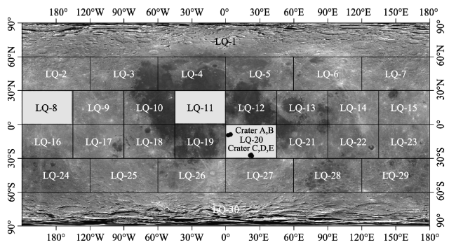
Figure 1 Map showing the locations of our study areas as well as the positions of selected craters

3 Methods

The classification algorithm used in this study includes DEM preprocessing, morphologic parameterization, ISO cluster unsupervised classification, and final landform map (Figure 2). Module implementation was designed to take advantage of publically available software packages in ArcGIS.
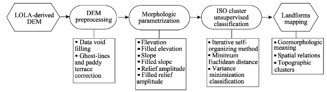
Figure 2 Flow chart illustrating the computational landform classification process applied in this study

3.1 DEM preprocessing

A DEM usually contains errors that need to be minimized before it can be utilized to extract terrain parameters. Thus, to mitigate external inputs, we corrected the DEM used in this study by lowering the elevation values of pixels around the model edges to correspond with the lowest recorded value for elevation (Tarboton et al., 1989) and completed the filling progress to address the issue of craters. We used the difference between filled and original elevation grids with non-zero values to represent pixels located within craters (O’Callaghan and Mark, 1984); the filled elevation process was completed using the sink, watershed, zonal statistics, zonal fill, and minus geoprocessing tools in the software program ArcGIS. Finally, because topographic analysis requires that a DEM is in a metric projection system, we converted GCS_MOON_2000 geographic coordinates to the Mercator projection.

3.2 Morphologic parameterization

In order to account for dichotomies (i.e., highlands and mares) and widely distributed impact craters on the surface of the Moon in our classification, we used six morphologic parameters (i.e., elevation, filled elevation, slope, filled slope, relief amplitude, and filled relief amplitude) to describe terrains derived from original and filled elevation fields. We initially derived slope and relief amplitude from the corrected DEM, and applied several algorithms to calculate topographic features. Because the results from different algorithms are closely correlated (Guth, 1995; Hodgson, 1998; Jones, 1998), we applied the formula proposed by Burrough and McDonnell (2011) to calculate slope and relief amplitude. Thus, filled slope and relief amplitude were calculated using the filled elevation field. However, because attributes stored in the different layers of our digital topography model (DTM) have different physical meanings and value ranges, we normalized original attribute values to a (0, 1) range so that all variables contribute equally to distances between different pixels. Note that a DEM is simply one kind of DTM in which layers encapsulate elevation values.

3.3 ISO cluster unsupervised classification

Unsupervised classifications utilize naturally occurring statistical groupings in data to determine clusters. We applied this approach to a series of input raster bands using ISO cluster and maximum likelihood classification tools (Kohonen, 1982). The ISO cluster algorithm is an iterative, self-organizing process for computing minimum Euclidean distance when assigning each candidate cell to a cluster. The process is initiated arbitrarily by the software in the case of each cluster, and every cell is assigned to the closest mean distance within the multidimensional attribute space. New means are then recalculated for each cluster based on the attributes of cells that belong to each after the first iteration, before the process is then repeated; each cell is again assigned to the closest mean within the multidimensional attribute space, and new means are calculated for each cluster based on the membership of cells from each iteration. As the number of iterations is a free parameter, we experimented with N = 12, N = 15, N = 20, and N = 40 clusters. Results show that clusters classify and display landforms at a level reasonably consistent with visual interpretation when N = 20, and that clusters merge with their neighbors when statistical values are similar after stability is reached. We used the Jenks natural breaks algorithm (Jenks and Caspall, 1971) to perform final merging; in this variance-minimization classification, within class variance is as small as possible while between class variance is as large as possible.

3.4 Landform mapping and interpretation

We automated the final result of our classification as a thematic landform map; assigning colors to different clusters enables the classification to be clearly visualized. Because initial cluster results are numerals that lack geomorphologic meaning, we replaced these labels with semantic ones by reviewing the statistical properties of the topographic characteristic in each cluster and studying the spatial relationships between clusters. This enabled us to determine which clusters correspond to specific landform classes as well as to compute and apply shaded relief to images for visualization purposes.

3.5 Confusion matrix

To determine the accuracy of our algorithm, we tested the result of each classification against a reference map (Fortezzo and Hare, 2013) using a confusion matrix. This kind of matrix is appropriate for use with traditional classification methods as it assumes that pixels at reference locations can be assigned to single classes; thus, accuracy measures based on the proportion of correctly classified area can be calculated via the number of correctly classified pixels (Lewis and Brown, 2001). The result of each classification and the reference map were converted to grid files of the same resolution and pixels were classified as either ‘crater’, ‘mare’, ‘lowland’, ‘highrelief’, or ‘highland’. These pixel classes were then assigned values of 0, 10, 20, 30, and 40 on the reference map and corresponding values of 0, 1, 2, 3, and 4 on the classification map. The two maps of the three test areas were then summed and a confusion matrix map constructed that comprised pixels with values ranging between 0 and 33. We then calculated overall accuracy (OA), producer accuracy (PA), user accuracy (UA), and the Kappa coefficient (K) based on values within the confusion matrix. Of these, OA measures the proportion of correctly classified reference pixels, while PA estimates the probability that a pixel of class i has been correctly assigned within the reference classification, UA refers to the probability that a pixel assigned to class i is actually a member of that group, and K measures the agreement between two classifications taking into account the possibility that coincidence can occur by chance (Cohen, 1960). Thus:
(1)
(2)
(3)
(4)
where n denotes the total number of reference pixels, k refers to the column, i refers to the row, po denotes relative observed agreement, and pe is the hypothetical probability of chance agreement. We computed confusion matrices and associated statistics using the software program ArcGIS 10.

4 Results

The values of topographic attributes averaged over pixels within each landform class for the three test areas are shown in Tables 1, 2, and 3. Average values where then used to construct a dendrogram of landform classes (Figure 3) that summarizes their degree of similarity. In these diagrams, classes that are more similar to one another are more closely connected; thus, Figure 3a shows that, of all possible pairs, class 2 and class 3 are most similar to one another, and also indicates that all 20 classes can be divided naturally into four larger groups which correspond to major landform types, A = (1, 2, 3, 4, 5, 6, 7, 8), B = (9, 10, 11, 12, 13), C = (14, 15, 16), and D = (17, 18, 19, 20). A thematic map constructed on the basis of this landform classification is shown in Figure 4. The different colors on this map denote pixel class membership; a physical interpretation was applied by reviewing the statistical and topographic attributes of pixels comprising each class and by studying their spatial relationships. The legends to Figures 4-6 summarize our interpretations; our results divide the 20 landform classes into five larger groups, encompassing mares, craters, lowlands, areas of highrelief, and highlands. This manual division, which also takes spatial relationships into account, closely corresponds with the algorithmic grouping shown in Figure 3 based only on the Euclidean distances between average attribute vectors.
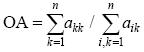
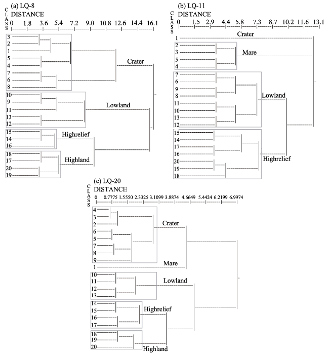
Figure 3 Dendrogram showing the relationships between the 20 landform classes generated by automatic classification within the LQ-8, LQ-11, and LQ-20 test areas. The gray rectangles denote the five major landform types identified manually by assigning geomorphologic interpretations to classes, while the multidimensional distance along the top of the dendrogram is the distance between classes in attribute space.
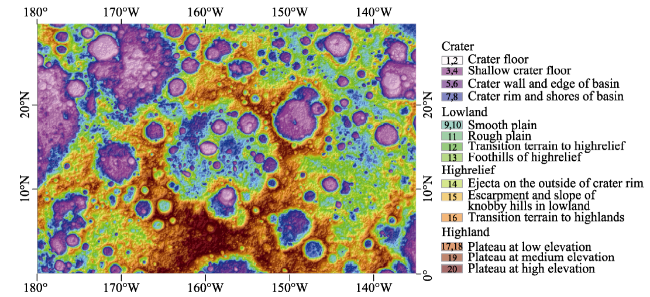
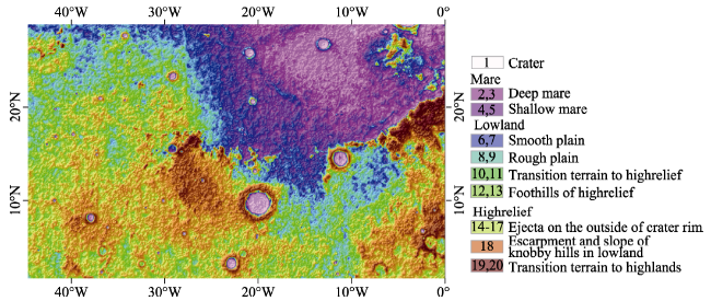
Figure 4 Thematic map showing automatically identified landforms within the LQ-8 test area. The geographic categories corresponding with numbered landform classes are outlined in the legend

4.1 LQ-8

Test area LQ-8 consists of cratered highlands that are not covered with basaltic lava. Results show that the topographic attributes of pixels in classes 1, 2, 3, 4, 5, 6, 7, and 8 are similar, with the exception that the signatures of large values for filled elevation that subdivide this range of topography comprise four distinct groups. Thus, pixels classified within classes 5 and 6 have higher slope values, perhaps the result of steeper inner crater walls, while pixels classified within classes 7 and 8 have the highest values of all for filled slope and relief, perhaps because the crater rim in these cases is elevated with respect to the adjacent lowland. As all these classes are identified as flat floors inside craters, crater walls, and crater rims, we classify them all together in this study within a larger group which we refer to as ‘craters’. Results show that 38.44% of pixels inside the LQ-8 test area can be classified within this group and that the major feature discriminating classes of craters are their values for filled elevation (Table 1).
Table 1 Average values for landform class morphologic parameters within the LQ-8 test area
Class Count
(pixels)
Elevation (m) Filled
elevation (m)
Slope (degree) Filled
slope (degree)
Relief
(m)
Filled relief (m)
1 106,694 -697 5787 6.17 6.17 1188 1187
2 262,266 512 4579 6.54 6.54 1245 1244
3 304,078 1216 3877 6.58 6.6 1262 1261
4 288,478 1794 3301 6.63 6.63 1263 1262
5 249,714 2257 2839 6.67 6.67 1270 1272
6 239,441 2618 2482 6.75 6.74 1272 1273
7 229,001 2890 2215 6.78 6.79 1275 1276
8 229,510 3112 2004 6.8 6.8 1278 1278
9 222,440 3306 1796 6.9 6.9 1291 1291
10 238,691 3491 1608 6.98 6.99 1297 1297
11 253,876 3676 1423 6.99 6.99 1306 1306
12 258,172 3864 1237 7.00 7.00 1314 1313
13 261,774 4062 1040 7.02 7.02 1318 1318
14 263,442 4281 821 7.03 7.03 1325 1325
15 281,458 4539 562 7.03 7.03 1325 1325
16 308,016 4864 235 7.04 7.04 1336 1336
17 325,804 5280 -182 7.24 7.25 1346 1346
18 316,858 5823 -723 7.31 7.32 1396 1395
19 224,284 6548 -1443 7.55 7.55 1412 1414
20 102,783 7743 -2634 7.74 7.75 1472 1472
The common characteristic of pixels in classes 9, 10, 11, 12, and 13 is their low relief; as all these pixels are spatially located below the escarpment, we collected them together into a larger group which we refer to as ‘lowland’. Results show that 24.21% of pixels within the LQ-8 test area can be classified within this group.
The pixels in classes 14, 15, and 16 are all located on highland at elevations in the vicinity of the escarpment; the common feature of all these pixels is a relatively similar slope value. Because the pixels in these groups collectively comprise an inter-crater plateau at relatively high elevations, we refer to them as ‘highrelief’. Results show that 17.17% of pixels inside the LQ-8 test area can be classified within this group.
The pixels in classes 17, 18, 19, and 20 all exhibit negative filled elevation values as well as higher values of slope, relief, and filled attributes. The pixels in these three classes are spatially located on highland, above the escarpment, and fill in the space between craters. These highland classes are mainly differentiated from one another by their filled elevation values; results show that 19.52% of pixels inside the LQ-8 test area can be classified as ‘highland’ (Figure 4).

4.2 LQ-11

The LQ-11 test area mainly comprises basaltic lava flows containing a few craters. The topographic attributes for pixels in class 1 within this area are unique because they exhibit the smallest values; pixels in this class are spatially located within concave pits that are separately distributed, filling their inner spaces. Because the spatial distribution of these class 1 pixels forms a number of hotspots, we collectively refer to them as ‘craters’; results show that just 0.86% of pixels inside the LQ-11 test area can be classified within this group (Table 2).
Table 2 Average values for landform class morphologic parameters within the LQ-11 test area
Class Count
(pixels)
Elevation (m) Filled elevation (m) Slope
(degree)
Filled
slope (degree)
Relief
(m)
Filled relief (m)
1 42,808 -3569 8776 1.85 1.86 337 337
2 265,504 -2766 7961 1.89 1.9 338 338
3 330,694 -2516 7709 1.91 1.91 342 341
4 313,714 -2306 7500 1.93 1.93 343 343
5 256,718 -2139 7334 1.93 1.93 344 345
6 192,104 -1996 7201 1.97 1.97 351 351
7 158,366 -1898 7091 1.99 1.99 352 352
8 156,600 -1808 6997 2.01 2.01 354 354
9 191,501 -1732 6921 2.01 2.01 358 358
10 228,543 -1662 6852 2.08 2.08 371 371
11 274,974 -1594 6787 2.2 2.18 383 383
12 320,671 -1528 6723 2.22 2.22 386 384
13 368,498 -1461 6656 2.23 2.23 398 398
14 414,463 -1389 6584 2.28 2.28 407 407
15 433,738 -1303 6497 2.62 2.62 455 455
16 411,237 -1184 6379 3.66 3.65 622 621
17 295,272 -999 6194 4.97 4.96 847 847
18 185,843 -680 5875 5.53 5.56 1116 1126
19 86,950 -152 5349 6.75 6.74 1248 1247
20 38,582 856 4344 7.95 7.95 1485 1484
The topographic attributes of pixels in classes 2, 3, 4, and 5 encompass a similar range as their elevation values range between -2800 m and -2000 m, their filled elevation values are all larger than 7200 m, their slopes are less than 1.95, and their relief values are all less than 350 m. The pixels in this class are spatially located in large and deep basins, and infill the inner space within basins which are often large, dark, basaltic plains formed by ancient volcanic eruptions. These pixels all correspond to a common landform type which we collectively refer to as ‘mare’. Results show that 23.49% of pixels inside the LQ-11 test area can be classified within this group (Figure 5).
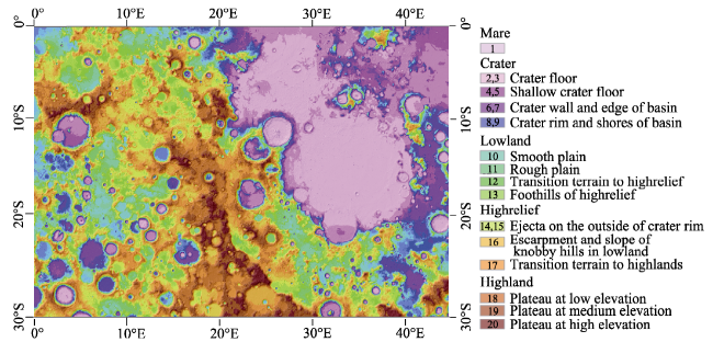
Figure 5 Thematic map showing automatically identified landforms within the LQ-11 test area. The geographic categories corresponding with numbered landform classes are outlined in the legend
The geomorphometric values of pixels within the range encompassed by class 6 to class 13 are slightly larger than those of the mare group and vary over smaller intervals. These pixels are all spatially located below the escarpment and represent the transitional zone between mare plains and regions of high slope and relief. These pixels are therefore collectively referred to as ‘lowland’; results show that 38.08% of pixels inside the LQ-11 test area can be classified within this group.
The pixels within the range encompassed by class 14 to class 20 are all located on highlands at high elevations in the vicinity of the escarpment. The pixels in these seven classes all share relatively high values of both slope and relief that vary over large intervals; taken together, they are indicative of an inter-mare plateau located on relatively highland while some represent ejecta on the outside of the crater rim. These pixels are collectively referred to as ‘highrelief’; results show that 37.57% of pixels inside the LQ-11 test area can be classified within this group.

4.3 LQ-20

The LQ-20 test area includes a greater diversity of landform units compared to its LQ-8 and LQ-11 counterparts. The topographic attributes for pixels in class 1 within this area are again unique (as above) because they exhibit the smallest values; these pixels are spatially located in large and deep craters and basins, filling their inner spaces, often large, dark, basaltic plains formed by ancient volcanic eruptions. As discussed above, these pixels are indicative of a common landform type which we collectively refer to as ‘mare’; results show that 14.81% of pixels inside the LQ-20 test area can be classified within this group (Table 3).
Table 3 Average values for landform class morphologic parameters within the LQ-20 test area
Class Count
(pixels)
Elevation (m) Filled elevation (m) Slope
(degree)
Filled
slope (degree)
Relief
(m)
Filled relief (m)
1 13,103,851 -5184 -184 6.84 6.84 272 287
2 7,767,995 -3749 1251 10.49 10.49 432 447
3 3,022,547 -3047 1953 10.92 10.92 460 481
4 3,932,609 -2584 2416 11.37 11.37 478 522
5 2,662,286 -2132 2868 12.70 12.70 540 668
6 2,023,806 -1779 3221 14.08 14.08 603 955
7 2,486,296 -1439 3561 13.53 13.53 581 1392
8 2,215,210 -1115 3885 13.47 13.44 581 2684
9 2,665,493 -821 2558 12.43 28.63 528 5942
10 3,546,739 -543 -3558 11.34 12.90 471 3494
11 4,014,407 -276 -3276 11.39 11.35 470 1489
12 4,133,915 -9 -3009 11.75 11.75 483 948
13 4,717,575 277 -2723 12.33 12.33 509 724
14 5,023,863 606 -2394 13.51 13.51 560 666
15 5,161,705 1012 -1988 14.22 14.22 593 646
16 5,667,975 1514 -1486 14.74 14.74 618 651
17 5,556,587 2166 -834 15.04 15.04 635 662
18 5,911,671 3045 45 15.28 15.28 650 678
19 3,473,170 4427 1427 16.50 16.50 707 748
20 1,368,136 6032 3032 16.74 16.74 722 762
The topographic attributes of pixels in classes 2, 3, 4, 5, 6, 7, 8, and 9 are similar, with the exception of the signatures of positive values of filled elevation that subdivide this topographic range into eight distinct regions. The pixels in these classes all exhibit small values for all topographic characteristics, with the exception of those in class 6 and class 9; those in class 6 are characterized by higher slope values which perhaps result from steep inner crater walls, while those in class 9 have the highest values for filled slope and relief, perhaps because their crater rims are higher than adjacent lowlands. The pixels in these classes are all identified as the flat floor inside craters, the crater wall, and the crater rim; we collect them all together within a larger group which we refer to here as ‘craters’. Results show that 30.27% of pixels inside the LQ-20 test site can be classified within this group and that they mainly differ from one another in filled elevation values.
The common characteristic of pixels in classes 10, 11, 12, and 13 is their low relief. These pixels are all located spatially below the escarpment and so are collected together in this study into a group that we refer to as ‘lowlands’. Results show that 18.55% of pixels inside the LQ-20 test site can be classified within this group (Figure 6).
Figure 6 Thematic map to show automatically identified landforms within the LQ-20 test area. The geographic categories corresponding with numbered landform classes are outlined in the legend
Pixels within classes 14, 15, 16, and 17 are all located on highlands at high elevations in the vicinity of the escarpment. The pixels within these four classes all share relatively high slope values; as they collectively form an inter-crater plateau located on relatively highlands, we refer to them as ‘highrelief’ in this study. Results show that 24.20% of pixels inside the LQ-20 test site can be classified within this group (Table 3).
The topographic attributes of pixels within classes 18, 19, and 20 are all very similar, with the exception of signatures that divide this high elevation range into three regions from the highest (class 20) to the lowest (class 18). The pixels in these classes all share large values for slope and filled attributes, and are located spatially on highlands, above the escarpment, and filling the space between craters. The major difference between these highland classes is their elevation values; results show that 12.16% of pixels inside the LQ-20 test site can be classified within this group.

5 Discussion

The results of this study show significant agreement between the results of automated classification and the reference map for the three test areas. Results reveal slightly higher OA and K values in area LQ-11 because just a few simple shaped craters with clear rims and a large area of mare plain are present in this region and are easily recognized. In contrast, OA and K values for area LQ-20 are the lowest because of the relatively complex landform types in this region. Values for UA and PA in the case of crater and mare morphologies are also relatively higher than for other landforms, while UA values for lowlands are also relatively high. The main explanation for these results is that this procedure assumes that craters have steep slopes, while mare plains occur at low elevation, and that lowland and highrelief regions are transitional areas with few distinctive geomorphometric characteristics. However, some old craters that have been heavily eroded can actually be as flat as the surrounding lava plains, while highreliefs that have been partly submerged by subsequent lava flows are also problematic as they cause exposed highrelief units to become less topographically distinct. Similarly, lava flows that have moved down steep highland slopes to form blankets pose a different problem because they form plains but will be classified incorrectly as lowlands (Table 4).
Table 4 Error matrix for the best classification result
Test area Landform UA% PA% OA% K
LQ-8 Crater 70.98 87.72 76.04 0.68
Mare - -
Lowland 86.4 85.1
Highrelief 85.41 56.79
Highland 64.24 81.72
LQ-11 Crater 61.53 97.45 83.34 0.77
Mare 85.04 82.95
Lowland 94.97 88.35
Highrelief 81.77 71.02
Highland - -
LQ-20 Crater 78.30 85.93 70.12 0.59
Mare 92.26 69.01
Lowland 77.54 68.62
Highrelief 53.31 67.24
Highland 76.09 87.81
Although visual inspection of the topographies shown on the thematic landform map (Figure 6) reveals that our classification is in close agreement overall with expectations, our automatic classification approach has nevertheless misclassified pixels in some regions because of the effects of aggradation (i.e., effusion and deposition) and degradation (i.e., erosion and deformation). Most of these misclassifications, however, occur on low, flat floors inside craters and on lowlands as the similarity measures we calculated between attribute vectors do not correspond to actual landform similarities. For example, infilling will have occurred within basins just up to the level of the lowest pour point around their edges; thus, a crater with undisturbed walls will have been filled to the rim and thus its internal pixels will be classified correctly, while one with a broken wall will be only partially filled and its internal pixels will be misclassified. Results suggest that the degree of misclassification will depend on the severity of the break; ghosted craters that lack clear boundaries will not be filled at all and so these pixels will be severely misclassified compared to other landscape types. To further discuss this issue, we selected three craters for closer examination, labeled A (3.96°E, 11.4°S), B (2.62°E, 11.9°S), and C (24.79°E, 28.33°S). Local views of these craters are shown in Figures 7a and 7b; the two panels of this figure illustrate the topography of these features via topographic contours superimposed onto thematic landform maps (Figure 7).
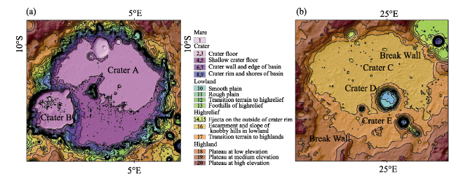
Figure 7 Local views of Crater A and Crater B (a), as well as Crater C, Crater D, and Crater E (b). Topographic contours have been superimposed onto landform maps in both cases; geographic categories corresponding with numbered landform classes are outlined in the legend
Images show that walls have mostly been damaged by erosion or by the superposition of other craters. The local view in Figure 7a shows that the walls of Crater A are broken in the 8 o’clock direction by Crater B. The pour point level is relatively high in this case, which means that most of the pixels on the crater floor are located beneath it and so are assigned to class 3 and class 4. However, some pixels on the rim of Crater B that are also on the flat floor of Crater A are also located below the pour point level and so are assigned to class 5 and class 6 rather than class 15 and class 16. Similarly, for the same reason, the pixels located on the walls of these craters will also be assigned to class 11 and class 12 rather than to class 15 and class 16. The small craters that comprise the deep basin within the flat floor of Crater A will also be assigned to class 1 because of their low elevation and maximal fill.
The local view of Crater C (Figure 7b) shows that this feature is also heavily eroded and has shallow walls that are broken in both 1 o’clock and 7 o’clock directions. The pour point level in this case is also very low, resulting in minimal fill; thus, most pixels in the interior of this crater will be assigned to highrelief class 17 and class 18 because they are located at high elevation. Results show that just a handful of deeper points will be classified as lowland and shallow crater floor within Crater D (25.12°E, 28.61°S) and Crater E (25.49°E, 29.15°S).

6 Conclusions

This study outlines an ISO cluster unsupervised classification approach for lunar landforms that is based on the hypothesis that each topographic entity on the Moon will be geomorphometrically distinct from the surrounding background. We test this approach using data for three representative lunar areas, LQ-8, LQ-11, and LQ-20. Numerous existing automated extraction approaches aim to identify and extract discrete landforms, including impact craters, valley networks, and other elements, by emphasizing their particular surface shapes; fewer, generically applicable, methodologies are available that evaluate the geometry of continuous surfaces (e.g., the whole lunar surface) and that are founded on statistical characterization. In this study, we have shown that our methodology is applicable by utilizing techniques drawn from the fields of data mining and artificial intelligence and applying them to planetary geomorphology. Thus, automated recognition of landforms can be achieved using our method at the local level of constituent pixels; each pixel in a continuous topography represented by a DEM is automatically classified by our ISO cluster unsupervised classification into one of 20 undefined landform types using the terrain parameters, elevation, filled elevation, slope, filled slope, relief amplitude, and filled relief amplitude. We chose an ISO cluster approach to generate initial groupings because of speed; ISO cluster processing of each DEM took approximately five minutes on a 2.50 GHz Core i3 machine for each test area.
Our results show that while elevation appears to be critical in recognizing highlands, filled elevation is of greater utility in distinguishing craters and mare plains. Subsequent to separating obvious landforms from other topographic features, our procedure then automatically adjusts the sensitivity of its criteria to accommodate subtler surface forms such as lowland and highrelief using filled slope and relief amplitude. In order to ensure statistically robust class definitions, thresholds for subdividing images are arbitrarily set as the mean values of frequency distributions and the signatures of input parameters. We quantitatively evaluated our approach using a series of confusion matrices and achieved overall accuracies as high as 83.34% and K values as high as 0.77. Our method represents a step forward because it is a reproducible and directly transferable approach to map lunar landforms; this technique can be performed easily using a GIS mapping platform, effortlessly edited, and incorporated into a general mapping procedure along with other landforms.
Automated classification generally results in less focused, more general purpose, thematic maps that incorporate broadly defined semantic meanings for landform classes. This reflects the unsupervised nature of the classifier; no landforms are defined beforehand and their meanings are established afterwards. Thus, the only available control over the emphasis placed on a landform is through choice of topographic attributes. In contrast, artificial landform classifications apply narrowly defined semantic definitions before mapping; thus, unsupervised landform classification facilitates automated searches for unexpected landscape features, while use of an automated classifier enables the quantitative determination of topographic similarities between different sites. Furthermore, the use of automated classification at the pixel level can delineate landscape features that exhibit detailed geomorphologic characteristics; lunar impact craters, for example, can be conveniently counted and described on the basis of constituent elements such as the crater rim, crater wall, ejecta, and central peak. We also tested the behavior of our classification system in this study, running it many times over the same dataset and generating identical results in each case. Results show that our classification system can accurately generate reproducible outputs, although further research will be required to establish optimal algorithm parameter values in a planetary context given the availability of high quality datasets, as well as to generate more complete terrestrial and planetary landform maps.

The authors have declared that no competing interests exist.

[1]
Adediran A O, Parcharidis I, Poscolieri Met al., 2004. Computer-assisted discrimination of morphological units on north-central Crete (Greece) by applying multivariate statistics to local relief gradients.Geomorphology, 58: 357-370. doi: 10.1016/j.geomorph.2003.07.024.Traditional manual methods have been employed for decades to measure geomorphometric properties from topographic maps. Such measurement techniques tend to be tedious and time-consuming and the designated landform elements cannot be easily overlaid on any digital map and imagery for further applied research. This study deals with a new quantitative geomorphometric procedure, based on the multivariate statistical analysis of local topographic gradients within a part of north-central Crete. This method employs sets of computer algorithms that automatically extract and classify geomorphometric properties from Digital Elevation Models (DEMs). This was done by evaluating the morphological setting around each pixel of the DEM along the eight azimuth directions. ISODATA unsupervised classification was implemented to generate 10 morphometric classes showing the spatial distribution of areas with a similar geomorphic scenario. Results revealed that this approach permitted a quick estimation of the spatial distribution of morphologically homogeneous terrain units. It also demonstrated the ability of the delineated landform elements to be superimposed on any digital map and imagery for further investigation. This became apparent during the examination of the relationship between the geomorphological units and the land-cover/land-use types in the study area. Both relative association and the dominant land cover/land use types in relation to geomorphological units are presented.

DOI

[2]
Bolongaro-Crevenna A, Torres-Rodriguez V, Sorani Vet al., 2005. Geomorphometric analysis for characterizing landforms in Morelos State, Mexico.Geomorphology, 67(3): 407-422. doi: 10.1016/j.geomorph.2004.11.007.Landforms can be described and quantified into simple relief elements by parametrization of digital elevation model (DEM). In this research, we investigate the use of morphometric parameters and a new classification scheme to characterize selected elemental forms associated with landforms. We apply and test this methodology on a geomorphologically diverse region located in Central Mexico. These simple elements are known as morphometric classes and include ridge, plane, channel, pit, peak, and pass. These classes correspond to real entities and are of practical significance. The morphometric classes were grouped according to their areal parameters (ridge, plane, and channel) and pointed parameters (pit, peak, and pass), which can be used to form the basis of a system of characterization and classification of landforms. Landform elements display statistically significant compositional differences with respect to their proportions of morphometric classes. This, in turn, can be plotted onto a diagram of characterization and classification known as a double ternary diagram (DTD), which comprises both areal and pointed parameters and any combination thereof. The DTD is useful for studying geomorphological processes wherein areal and point values and properties have expressions which are topographically quantifiable.

DOI

[3]
Bue B D, Stepinski T F, 2006. Machine detection of Martian craters from digital topography. In: 37th Annual Lunar and Planetary Science Conference, 37: 1178.An automated crater detection algorithm based on Martian DEM data is developed and its performance is compared to the image-based catalog of Martian craters manually compiled by N. Barlow.

[4]
Burrough P A, McDonnell R A, 2011. Principles of Geographical Information Systems (Vol. 19988). Oxford: Oxford University Press.

[5]
Burrough P A, Gaans P F M V, Macmillan R A, 2000. High-resolution landform classification using fuzzy k-means.Fuzzy Sets and System, 113(1): 37-52. doi: 10.1016/S0165-0114(99)00011-1.

DOI

[6]
Butle D R, Walsh S J, 1998. The application of remote sensing and geographic information systems in the study of geomorphology: An introduction.Geomorphology, 21(3): 179-181. doi: 10.1016/S0169-555X(97)00056-1.Not Available

DOI

[7]
Cohen J, 1960. A coefficient of agreement for nominal scales.Educational and Psychological Measurement, 20(1): 37-46. doi: 10.1177/001316446002000104.A Coefficient of agreement for nominal Scales COHEN J. Educational and Psychological Measurement 20(1), 37-46, 1960

DOI

[8]
Dehn M, Gärtner H, Dikau R, 2001. Principles of semantic modeling of landform structures.Computer Geoscience, 27: 1005-1010. doi: 10.1016/S0098-3004(00)00138-2.Landforms, which result from the interplay of physical, chemical, and biological processes acting on the surface, function as static boundary conditions for processes in geomorphology, hydrology, meteorology and other fields. The description, parameterization, and modeling of landform structure, as well as the terminology used, are fitted to the requirements of the disciplines and are, therefore, often strongly divergent. As a consequence, representations of landform structure for different disciplines are often not compatible and require frequent revisions and adaptations. Principles of the semantic approach to the problem are presented in this paper. The main objective is a semantically correct description of landform which is useful to all disciplines related to surface structure. The approach considers geometric form as a basic property, extended by topological considerations and semantic definitions. The potential, limitations, and open questions of the semantic-based approach are discussed using hillslopes as a case study. The focus of the paper is on semantic representation and only thereafter are the special features of DEMs, tools, and implementations considered.

DOI

[9]
Drăguţ L, Blaschke T, 2006. Automated classification of landform elements using object-based image analysis.Geomorphology, 81(3): 330-344. doi: 10.1016/j.geomorph.2006.04.013.This paper presents an automated classification system of landform elements based on object-oriented image analysis. First, several data layers are produced from Digital Terrain Models (DTM): elevation, profile curvature, plan curvature and slope gradient. Second, relatively homogenous objects are delineated at several levels through image segmentation. These object primatives are classified as landform elements using a relative classification model, built both on the surface shape and on the altitudinal position of objects. So far, slope aspect was not used in classification. The classification has nine classes: peaks and toe slopes (defined by the altitudinal position or the degree of dominance), steep slopes and flat/gentle slopes (defined by slope gradients), shoulders and negative contacts (defined by profile curvatures), head slopes, side slopes and nose slopes (defined by plan curvatures). Classes are defined using flexible fuzzy membership functions. Results are visually analyzed by draping them over DTMs. Specific fuzzy classification options were used to obtain an assessment of output accuracy. Two implementations of the methodology are compared using (1) Romanian datasets and (2) Berchtesgaden National Park, Germany. The methodology has proven to be reproducible; readily adaptable for diverse landscapes and datasets; and useful in respect to providing additional information for geomorphological and landscape studies. A major advantage of this new methodology is its transferability, given that it uses only relative values and relative positions to neighboring objects. The methodology introduced in this paper can be used for almost any application where relationships between topographic features and other components of landscapes are to be assessed.

DOI

[10]
Ehlers M, Janowsky R, Gaehler M, 2002. New remote sensing concepts for environmental monitoring. In: International Society for Optics and Photonics. International Symposium on Remote Sensing, 1-12.The availability of remote sensing data that are needed for global, regional and local environmental monitoring has greatly increased over the recent years. New technologies such as global positioning system (GPS), digital photogrammetry and multi-source satellite remote sensing are creating data at higher spatial, spectral and temporal resolution than have been collected at any other time on earth. Geographic Information Systems (GIS) technologies allow - for the first time- the efficient storage and management of spatial datasets in digital formats. In combination with the appropriate data transfer and interoperability standards that are currently being developed the technology is being put in place that will eventually allow standardized data exchange, processing and dissemination. Today, a wide variety of remote sensing systems are used to provide information about the earth, its atmosphere, oceans, and land surfaces. Multispectral satellite scanners in the visible and near infrared domains of the electromagnetic spectrum record solar radiation reflected from the earth's surface. Data derived from multispectral scanners provide information on (among other things): vegetation type, distribution and condition; geomorphology; soils; surface waters; and river networks. In addition, active microwave (radar) systems are commonly used in geological, hydrological and oceanographic applications. The advent of very high resolution satellite and space programs offers new possibilities for satellite remote sensing. In addition, digital airborne cameras offer ultra high resolution for very accurate mapping of the environment.

DOI

[11]
Florinsky I V, 1998. Accuracy of local topographic variables derived from digital elevation models.International Journal of Geographical Information Science, 12(1): 47-62. doi: 10.1080/136588198242003.We study the accuracy of data on some local topographic attributes derived from digital elevation models (DEMs). First, we carry out a test for the precision of four methods for calculation of partial derivatives of elevations. We find that the Evans method is the most precision algorithm of this kind. Second, we produce formulae for root mean square errors of four local topographic variables (gradient, aspect, horizontal and vertical landsurface curvatures), provided that these variables are evaluated with the Evans method. Third, we demonstrate that mapping is the most convenient and pictorial way for the practical implementation of the formulae derived. A DEM of a part of the Kursk Region (Russia) is used as an example. We find that high errors of data on local topographic variables are typical for flat areas. Results of the study can be used to improve landscape investigations with digital terrain models.

DOI

[12]
Fortezzo C M, Hare T M, 2013. Completed digital renovation of the 1:5,000,000 lunar geologic map series. Lunar and Planetary Science Conference, Vol. 44.We have completed digitizing the 1:5M-scale lunar maps to LOLA and WAC global basemaps and have them available for use in geographic information system formats.

[13]
Gaddis L R, Skinner J A J, Hare T et al., 2006.The lunar geologic mapping program and status of Copernicus quadrangle mapping. In: 37th Annual Lunar and Planetary Science Conference, Vol. 37, p.2135.We are mapping a lunar quadrangle at 1:2.5M scale that centers on Copernicus crater.

[14]
Giles P T, Franklin S E, 1998. An automated approach to the classification of the slope units using digital data.Geomorphology, 21(3): 251-264. doi: 10.1016/S0169-555X(97)00064-0.Digital elevation and remote sensing data sets contain different, yet complementary, information related to geomorphological features. Digital elevation models (DEMs) represent the topography, or land form, whereas remote sensing data record the reflectance/emittance, or spectral, characteristics of surfaces. Computer analysis of integrated digital data sets can be exploited for geomorphological classification using automated methods developed in the remote sensing community. In the present study, geomorphological classification in a moderate- to high-relief area dominated by slope processes in southwest Yukon Territory, Canada, is performed with a combined set of geomorphometric and spectral variables in a linear discriminant analysis. An automated method was developed to find the boundaries of geomorphological objects and to extract the objects as groups of aggregated pixels. The geomorphological objects selected are slope units, with the boundaries being breaks of slope on two-dimensional downslope profiles. Each slope unit is described by variables summarizing the shape, topographic, and spectral characteristics of the aggregated group of pixels. Overall discrimination accuracy of 90% is achieved for the aggregated slope units in ten classes.

DOI

[15]
Guth P L, 1995. Slope and aspect calculations on gridded digital elevation models: Examples from a geomorphometric toolbox for personal computers.Zeitschrift fur Geomorphologie Supplementband, 101: 31-52.Abstract The power of microcomputers and availability of digital data bring morphometry within the reach of all earth scientists. The MICRODEM program provides a general purpose tool box for digital elevation models (DEMs). Six different algorithms have been used to compute slope and aspect, all considering a point and up to eight surrounding elevations. Even with the large 45 aspect categories, the best resolution provided by some algorithms, the methods do not give consistent estimates of downhill direction, and all methods display undue clustering of aspect in the eight principal compass directions. -from Author

[16]
Hengl T, Rossiter D G, 2003. Supervised landform classification to enhance and replace photo-interpretation in semi-detailed soil survey.Soil Science Society of America Journal, 67: 1810-1822. doi: 10.2136/sssaj2003.1810.A method to enhance manual landform delineation using photo-interpretation to map a larger area is described. Conventional aerial photo-interpretation (API) maps using a geo-pedological legend of 21 classes were prepared for six sample areas totaling 111 km&sup2 ; ; ; in Baranja region, eastern Croatia. Nine terrain parameters extracted from a digital elevation model (ground water depth, slope, plan curvature, profile curvature, viewshed, accumulation flow, wetness index, sediment transport index and the distance to nearest watercourse) were used to extrapolate photo-interpretation over the entire survey area (1062 km&sup2 ; ; ; ). The classification accuracy was assessed using the error matrix, calculated by comparing both the whole API maps and point samples, with the results of classification. The first results, using a maximum-likelihood classifier, were 58.2% (hill land), 39.1% (plain), and 45.3% (entire area) reproducibility of the training set. Six classes in the plain were responsible for a large proportion of the misclassifications, due to an insufficiently detailed digital elevation model and the complex nature of landforms (point bar complexes, levees, active channel banks), which can not be explained with the terrain parameters only. Reproducibility for a simplified legend of 15 classes over the study area was improved to 65.8% (plain), 58.2% (hill land) and 63.4% (entire area) using the whole-API training set. After the simplification of legend (15) and with the iterative (3) selection of point-sample training set, classification was able to reproduce 97.6% (hill land), 86.7% (plain), and 90.2% (entire area) of the training set. The supervised classification showed fine details not achieved by photo-interpretation. The number of manual photo-interpretations that had to be prepared was reduced from 84 to 6. The methodology can be applied by soil survey teams to edit and update current maps and to enhance or replace API for new surveys.

DOI

[17]
Hodgson M E, 1998. Comparison of angles from surface slope/aspect algorithms.Cartography and Geographic Information Systems, 25(3): 173-185. doi: 10.1559/152304098782383106.Few studies have compared algorithms for mapping surface slope and aspect from digital elevation models. Those studies that have compared these algorithms treat slope and aspect angles independently. The evaluation and comparison of surface orientation algorithms may also be conducted by treating slope and aspect as characteristics of a bi-directional vector normal to the surface. Such a comparison is more appropriate for selecting an accurate surface orientation algorithm for applications that use bi-directional measurements, such as modeling solar radiation or removing the topographic effect from remotely sensed imagery. This study empirically compared the slope angle and bi-directional surface angle estimated from five slope/aspect algorithms using a synthetic terrain surface and an actual terrain surface. The most accurate algorithm is consistently that which uses only the four nearest neighboring elevations in the grid.

DOI

[18]
Iwahashi J, Pike R J, 2007. Automated classifications of topography from DEMs by an unsupervised nested-means algorithm and a three-part geometric signature.Geomorphology, 86: 409-440. doi: 10.1016/j.geomorph.2006.09.012.An iterative procedure that implements the classification of continuous topography as a problem in digital image-processing automatically divides an area into categories of surface form; three taxonomic criteria lope gradient, local convexity, and surface texture re calculated from a square-grid digital elevation model (DEM). The sequence of programmed operations combines twofold-partitioned maps of the three variables converted to greyscale images, using the mean of each variable as the dividing threshold. To subdivide increasingly subtle topography, grid cells sloping at less than mean gradient of the input DEM are classified by designating mean values of successively lower-sloping subsets of the study area (nested means) as taxonomic thresholds, thereby increasing the number of output categories from the minimum 8 to 12 or 16. Program output is exemplified by 16 topographic types for the world at 1-km spatial resolution (SRTM30 data), the Japanese Islands at 270m, and part of Hokkaido at 55m. Because the procedure is unsupervised and reflects frequency distributions of the input variables rather than pre-set criteria, the resulting classes are undefined and must be calibrated empirically by subsequent analysis. Maps of the example classifications reflect physiographic regions, geological structure, and landform as well as slope materials and processes; fine-textured terrain categories tend to correlate with erosional topography or older surfaces, coarse-textured classes with areas of little dissection. In Japan the resulting classes approximate landform types mapped from airphoto analysis, while in the Americas they create map patterns resembling Hammond's terrain types or surface-form classes; SRTM30 output for the United States compares favorably with Fenneman's physical divisions. Experiments are suggested for further developing the method; the Arc/Info AML and the map of terrain classes for the world are available as online downloads.

DOI

[19]
Jenks G F, Caspall F C, 1971. Error on choroplethic maps: Definition, measurement, reduction.Annals of the Association of American Geographers, 61(2): 217-244. doi: 10.1111/j.1467-8306.1971.tb00779.x.

DOI

[20]
Jones K H, 1998. A comparison of algorithms used to compute hill slope as a property of the DEM.Computer Geoscience, 24: 315-324. doi: 10.1016/S0098-3004(98)00032-6.The calculation of hill slope in the form of downhill gradient and aspect for a point in a digital elevation model (DEM), is a popular procedure in the hydrological, environmental and remote sensing. The most commonly used slope calculation algorithms employed on DEM topography data make use of a three by three search window, or kernel, centred on the grid point (grid cell) in question in order to calculate the gradient and aspect at that point. A comparison of eight frequently used slope calculation algorithms for digital elevation matrices has been carried out using both synthetic and real data as test surfaces. Morrison's surface III, a trigonometrically defined surface, was used as the synthetic test surface. This was differentiated analytically to give true gradient and aspect values against which to compare the results of the tested algorithms. The results of the best-performing slope algorithm on Morrison's surface were then used as the reference against which to compare the other tested algorithms on a real DEM. For both of the test surfaces residual gradient and aspect grids were calculated by subtracting the gradient and aspect grids produced by the algorithms on test from the true/reference gradient and aspect grids. The resulting residual gradient and aspect grids were used to calculate root-mean-square (RMS) residual error estimates that were used to rank the slope algorithms from “best” (lowest value of RMS residual error) to “worst” (largest value of RMS residual error). For Morrison's test surface, Fleming and Hoffer's method gave the “best” results for both gradient and aspect. Horn's method (used in ArcInfo GRID) also performed well for both gradient and aspect estimation. However, the popular maximum downward gradient method (MDG) performed poorly, coming last in the rankings. A similar pattern was seen in the gradient and aspect rankings derived using the Rhum DEM, with Horn's method performing well and the MDG method poorly.

DOI

[21]
Kohonen T, 1982. Self-organized formation of topologically correct feature maps.Biological Cybernetics, 43(1): 59-69. doi: 10.1016/S0925-2312(98)00030-7.

DOI

[22]
Lewis H G, Brown M, 2001. A generalized confusion matrix for assessing area estimates from remotely sensed data. International Journal of Remote Sensing, 22(16): 3223-3235. doi: 10.1080/01431160152558332.The formulation of a generalized area-based confusion matrix for exploring the accuracy of area estimates is presented. The generalized confusion matrix is appropriate for both traditional classification algorithms and sub-pixel area estimation models. An error matrix, derived from the generalized confusion matrix, allows the accuracy of maps generated using area estimation models to be assessed quantitatively and compared to the accuracies obtained from traditional classification techniques. The application of this approach is demonstrated for an area estimation model applied to Landsat data of an urban area of the United Kingdom.

DOI

[23]
Miliaresis G C, 2001. Extraction of bajadas from digital elevation models and satellite imagery.Computer Geoscience, 27(10): 1157-1167. doi: 10.1016/S0098-3004(01)00032-2.A methodology was designed for the extraction of bajadas from the ja:math US Geological Survey digital elevation models and Landsat Thematic Mapper imagery. The method was demonstrated for the Death Valley-California where progressive eastward tilting has enabled the west-side fans to coalesce and form bajadas. First, the drainage that crossed the uplands and the bajadas was extracted from the DEM. The drainage pixels were successively grown by checking the surrounding pixels on the basis of their gradient. It was concluded that for gradient in the interval [2 ,11 ] the upslope bajadas border was segmented. In order to eliminate the drainage pixels that belonged to the uplands, the drainage pixels were subtracted. Then, the isolated small 8-connected foreground pixels were identified and subtracted too. Finally, region growing was performed again to the remaining pixels with the same growing criterion. Isolated 8-connected background pixels, representing almost flat regions inside bajadas, were identified and merged to the segmented pixels. At the end, by taking into account the spectral response in the satellite image, the downslope border of bajadas was segmented. The extracted polygon was in agreement with the information depicted on (a) the US Geological Survey topographic map of scale 1:100,000 and (b) the satellite image and (c) the polygon classified manually by a photo-interpreter.

DOI

[24]
O'Callaghan J F, Mark D M, 1984. The extraction of drainage networks from digital elevation data. Computer Vision, Graphics,and Image Processing, 28(3): 323-344. doi: 10.1016/S0734-189X(84)80011-0.The extraction of drainage networks from digital elevation data is important for quantitative studies in geomorphology and hydrology. A method is presented for extracting drainage networks from gridded elevation data. The method handles artificial pits introduced by data collection systems and extracts only the major drainage paths. Its performance appears to be consistent with the visual interpretation of drainage patterns from elevation contours.

DOI

[25]
Prima O D A, Echigo A, Yokoyama Ret al., 2006.Supervised landform classification of Northeast Honshu from DEM-derived thematic maps.Geomorphology, 78: 373-386. doi: 10.1016/j.geomorph.2006.02.005.This paper proposes a quantitative method to classify landforms using four morphometric parameters from DEM-derived thematic raster maps of slope and topographic openness. Because the different surficial processes and stages in the evolution of slopes create landscapes with different shapes, these parameters may lead to a genetic interpretation of topography. The raster maps of slope and topographic openness were constructed for Northeast Honshu, Japan, from 50-m DEMs. The mean and standard deviation of morphometric parameters within a 3050 m by 3050 m moving window on the raster maps were calculated. The results for some training areas show that constructional/depositional and erosional landforms with different relief have different morphometric characteristics. A supervised landform classification for Northeast Honshu using the knowledge from the training areas revealed a ladder geomorphological structure composed of high mountains, ranges and volcanoes. The close relationship between the ladder geomorphological structure and volcano distribution indicates that the structure reflects the magmatic plumbing system from the upper mantle to the crust of the Northeast Honshu arc.

DOI

[26]
Smith D E, Zuber M T, Jackson G Bet al., 2010. The lunar orbiter laser altimeter investigation on the lunar reconnaissance orbiter mission. Space Science Review, 150(1-4): 209-241. doi: 10.1007/s11214-009-9512-y.The Lunar Orbiter Laser Altimeter (LOLA) is an instrument on the payload of NASA’s Lunar Reconnaissance Orbiter spacecraft (LRO) (Chin et al., in Space Sci. Rev. 129:391–419, 2007 ). The instrument is designed to measure the shape of the Moon by measuring precisely the range from the spacecraft to the lunar surface, and incorporating precision orbit determination of LRO, referencing surface ranges to the Moon’s center of mass. LOLA has 5 beams and operates at 28 Hz, with a nominal accuracy of 10 cm. Its primary objective is to produce a global geodetic grid for the Moon to which all other observations can be precisely referenced.

DOI

[27]
Stepinski T F, Collier M L, 2004. Extraction of Martian valley networks from digital topography. Journal of Geophysical Research, Planets, 109(E11): 179-204. doi: 10.1029/2004JE002269.We have developed a novel method for delineating valley networks on Mars. The valleys are inferred from digital topography by an autonomous computer algorithm as drainage networks, instead of being manually mapped from images. Individual drainage basins are precisely defined and reconstructed to restore flow continuity disrupted by craters. Drainage networks are extracted from their underlying basins using the contributing area threshold method. We demonstrate that such drainage networks coincide with mapped valley networks verifying that valley networks are indeed drainage systems. Our procedure is capable of delineating and analyzing valley networks with unparalleled speed and consistency. We have applied this method to 28 Noachian locations on Mars exhibiting prominent valley networks. All extracted networks have a planar morphology similar to that of terrestrial river networks. They are characterized by a drainage density of ~0.1 km, low in comparison to the drainage density of terrestrial river networks. Slopes of ``streams'' in Martian valley networks decrease downstream at a slower rate than slopes of streams in terrestrial river networks. This analysis, based on a sizable data set of valley networks, reveals that although valley networks have some features pointing to their origin by precipitation-fed runoff erosion, their quantitative characteristics suggest that precipitation intensity and/or longevity of past pluvial climate were inadequate to develop mature drainage basins on Mars.

DOI

[28]
Stepinski T F, Vilalta R, 2005. Digital topography models for Martian surfaces.IEEE Geoscience and Remote Sensing Letters, 2(3): 260-264. doi: 10.1109/LGRS.2005.848509.We propose to use an unsupervised automated classification of topographic features on Mars in order to speed up geomorphic and geologic mapping of the planet. We construct a digital topography model (DTM), a multilayer grid that stores various kinds ...

DOI

[29]
Tarboton D G, Bras R L, Rodriguez-Iturbe I, 1989. The analysis of river basins and channel networks using digital terrain data. Technical Report No. 326, Ralf M. Cambridge: Parsons Laboratory, MIT.Thesis (Sc. D.)--Massachusetts Institute of Technology, Dept. of Civil Engineering, 1990.Vita.Includes bibliographical references (p. 210-220).

[30]
Wang J, Cheng W M, Zhou C H, 2015. A Chang’E global catalog of lunar impact craters.Planet Space Science, 112: 42-45. doi: 10.1016/j.pss.2015.04.012.61Detected lunar impact craters with diameters more than 500m using Chang'E-1 data in a hybrid method.61Compiled a global catalog of 106016 impact craters with comprehensive morphometric parameters.61Inspected the asymmetric spatial distribution of impact craters.

DOI

[31]
Wessel P, Smith W H, 2001. The Generic Mapping Tools. .

Outlines

/