4.1.1 Quantitative estimation of urban construction land
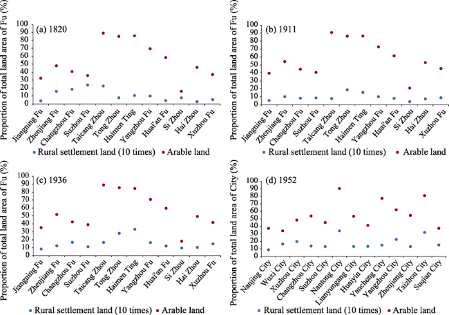
Cities and towns are highly concentrated with population, resources, environment, and socio-economic elements. Urban construction land expands along with the development of any of these elements. Such expansion has the characteristics of temporal sequentiality, periodicity, irreversibility, and spatial particularity. Between 1820 and 1911, the urbanization level (i.e., the proportion of urban population) was maintained at around 10% (
Li and Xu, 2008). Most cities were political centers established by the governments and had specially constructed boundary walls. Therefore, it is quite anticipated that the urban population density might fluctuate gradually within city walls and so does the value of per capita urban construction land, the estimation of urban construction land by using data such as city walls and four gates along walls can escape meddles with population changes.
In this study, urban construction land in 1820 is estimated mainly based on the perimeter and shape of city/town walls. Data of four gates along the walls and the land vacancy ratio representing arable land and open space that was present within the walls are also used in case for calibration. Moreover, the estimation of the urban construction land at the Fu (city) level also takes the special form of urban administrative divisions (for example, “Fu” and “County” in the same city, or multiple counties within the same city) (
Jin et al., 2016) into consideration. Such estimation has been conducted as in Equation 1:
$\left\{ \begin{align}& {{A}_{i}}=\sum\limits_{j=1}^{s}{A{{U}_{ji}}} \\& A{{U}_{ji}}={{L}_{ji}}\times {{W}_{ji}}\times \left( 1{{\alpha }_{ji}} \right) \\& {{L}_{ji}}={{W}_{ji}}=\frac{{{P}_{ji}}}{4} \\ \end{align} \right.$
$A_i$ is the area of urban construction land in Fu $ i$;
s is the number of cities/towns in Fu $ i$;
$ AU_{ji}$ is the area of construction land in city/town j of Fu $ i$;
$L_{ji}$ and $W_{ji}$ are the length and width of the border of city/town j in Fu $ i$, respectively;
$\alpha_{ji}$ is the vacancy ratio in the border of wall in city/town j of Fu $ i$; and
$P_{ji}$ is the perimeter of the walls of city/town j in Fu $ i$.
The unified form of a city/town is set as rectangular.
Referred to cities/towns in the south of the Yangtze River that have rich data about four gates (
Fan, 1990), the length×width ($L_{i}\times W_{i}$) of a large town is defined at 3.75×10
6 m
2, a medium town at 2.5×10
6 m
2, and a small town at 2.5×10
5 m
2. $\alpha$ for a provincial capital is set at 65% (
Cao et al., 1997), that for a normal Fu is 50%, and that for a county/town is 40%. In cases where overlay occurs, Fu takes the priority in area allocation, i.e., the area will be assigned to Fu but not county; and only one county will have the allocation if more counties than one are located within the same city.
The development of society, economy and politics leads to changes in the size and structure of population, and in sequence effects on the demand for land resources, i.e., for residence, production, and business activities. In the early modern period, it is more obvious for the city/town walls to act as the restriction to urban development. Urban construction land progressively broke through the walls and expanded greatly. In this study, the construction land in recent and early modern periods (i.e., in 1911, 1936 and 1952) has been estimated and calculated based on the population size and structure as in equations 2-5.
$\left\{ \begin{align} & {{A}_{i\left( t \right)}}=\sum\limits_{j=c,z}{A{{P}_{ji\left( t \right)}}\times {{P}_{Ti\left( t \right)}}\times {{\beta }_{ji\left( t \right)}}\left( t=1,2,3 \right)} \\ & A{{P}_{ui\left( t \right)}}=A{{P}_{ci\left( t \right)}}=A{{P}_{zi\left( t \right)}} \\ \end{align} \right.$ (2)
$A{{P}_{ui\left( t \right)}}=\left\{ \begin{align} & A{{P}_{ui\left( t-1 \right)}}+\left( A{{P}_{\overline{us}\left( t \right)}}-A{{P}_{ui\left( t-1 \right)}} \right)\times {{N}_{i\left( t \right)}},t=1,2,3 \\ & \frac{{{A}_{i\left( t \right)}}}{{{N}_{\overline{up}i\left( t \right)}}},t=0 \\ \end{align} \right.$ (3)
$A{{P}_{\overline{us}\left( t \right)}}=\frac{1}{n}\sum\limits_{m=1}^{n}{\frac{{{L}_{m}}\times {{W}_{m}}}{{{H}_{m\left( t \right)}}\times {{P}_{Hm\left( t \right)}}}}$ (4)
${{N}_{i\left( t \right)}}={\frac{{{N}_{\overline{uc}i\left( t \right)}}}{{{N}_{\overline{up}i\left( t \right)}}}}/{\left( \frac{1}{k}\sum\limits_{m=1}^{k}{\frac{{{N}_{\overline{uc}m\left( t \right)}}}{{{N}_{\overline{up}m\left( t \right)}}}} \right)}\;$ (5)
$A_{i(t)}$ is the area of urban construction land of Fu $i$ in the period of $t$;
$AP_{ui(t)}$, $AP_{ci(t)}$, and $AP_{zi(t)}$ represent per capita land use of urban, city and town of Fu $i$ in the period of $t$, respectively;
$P_{Ti(t)}$ is the total population size of Fu $i$ in the period of $t$;
$\beta_{ji(t)}$ is the population structure of Fu $i$ in the period of $t$;
$AP_{ui(t-1)}$ is the per capita urban construction land of Fu $i$ in the period of $t-1$;
$A{{P}_{\overline{us}\left( t \right)}}$ is the average value of per capita urban construction land in the period $t$;
Ni(t) is the urban socio-economic modification indicators of Fu $i$ in the period of $t$;
t=0, 1, 2 and 3 represent the year 1820, 1911, 1936 and 1952, respectively;
$H_{m(t)}$ is the number of households within city/town $m$ in the period of $t$;
$P_{Hm(t)}$ is the average household population of city/town $m$ in the period of $t$;
n is the number of cities and towns in Jiangsu in the period of $t$;
${{N}_{\overline{uc}i\left( t \right)}}$ is the urban socio-economic indicators of Fu $i$ in the period of $t$;
${{N}_{\overline{up}i\left( t \right)}}$ is the urban population of Fu $i$ in the period of $t$;
$\frac{1}{k}\sum\limits_{m=1}^{k}{\frac{{{N}_{\overline{uc}m\left( t \right)}}}{{{N}_{\overline{up}m\left( t \right)}}}}$ is the average value of per capita urban socio-economic indicators in the period of t; and
$k$ is the number of Fu in Jiangsu in the period of $t$.
Population in most counties grows and diffuses into surrounding areas. Per capita urban construction land is estimated based on the land area within the walls and population within cities/towns. Per capita urban construction land in each city/town is then amended with the number of business associations and chamber of commerce in the city.
(3) In the years 1936 and 1952
In the middle period of the Republic of China, factories gathered in cities and towns and the national capital began to emerge. During the Anti-Japanese War (1937-1945), all cities in Jiangsu were invaded more or less. Transportation system collapsed, industrial factories were occupied and the handicraft industry had almost been halted. Urban development in this period was in a stagnant status. From the end of the WWII to 1949, the urban population had increased and the urban development had recovered.
Assuming that the urban development level in 1936 was equivalent to that in 1952, per capita urban construction land can be determined based on data in 1952. Per capita urban gross value of products in 1936 can be used to fine calibrate such base data to reflect variations in economies and urban development across regions in 1936. Similarly, per capita added value of the secondary and tertiary industries in 1952 can be utilized as socio- economic indicators as well to refine the base data to evidence the imbalance across regions in 1952.
4.1.2 Quantitative estimation of rural settlement land
The village is an important component of the settlement system. Rural settlements were initially connected by affinities or clans and formed slowly and stably. The amount and distribution of rural settlement land is affected by the population, family structure, life style, as well as terrain, water resources, and cultivation radius. In general, they were not separated by defined spatial physical barriers (such as city/town walls). The form of social function is generally simple in rural areas. The relationship between the population and arable land affected the evolution of rural settlements. Compared with the urban land, the rural settlement land is expected to be positively correlated with the rural population.
In this study, the rural settlement land area in each period is estimated based on the population size, per capita land area and residential forms as in equations 6-11.
$A{{R}_{i\left( t \right)}}=A{{P}_{ri\left( t \right)}}\times {{P}_{TRi\left( t \right)}}$ (6)
$A{{P}_{ri\left( t \right)}}={A{{P}_{bi\left( {{t}_{0}} \right)}}}/{{{\lambda }_{i\left( t \right)}}}\;$ (7)
$A{{P}_{bi\left( {{t}_{0}} \right)}}={A{{P}_{hi\left( {{t}_{0}} \right)}}}/{R{{C}_{i\left( {{t}_{1}} \right)}}}\;$ (8)
$A{{P}_{hi\left( {{t}_{0}} \right)}}={A{{H}_{hi\left( {{t}_{0}} \right)}}}/{{{P}_{Fi\left( {{t}_{0}} \right)}}}\;$ (9)
${{\lambda }_{i\left( t \right)}}=\left\{ \begin{align} & 1,\text{ }t=0 \\ & {{\lambda }_{h\left( t \right)}}\left( {{\lambda }_{h\left( t \right)}}{{\lambda }_{l\left( t \right)}} \right)\times N{{R}_{i\left( t \right)}},\text{ }t=1,2,3 \\ \end{align} \right.$ (10)
$N{{R}_{i\left( t \right)}}={\frac{{{N}_{\overline{rc}i\left( t \right)}}}{{{N}_{\overline{rp}i\left( t \right)}}}}/{\left( \underset{m=1,2,\cdots ,k}{\mathop{\max }}\,\left\{ \frac{{{N}_{\overline{rc}m\left( t \right)}}}{{{N}_{\overline{rp}m\left( t \right)}}} \right\} \right)}\;$ (11)
$AR_{i(t)}$ is the area of rural settlement land of Fu i in the period of t;
$R_{TRi(t)}$ is the rural population size of Fu i in the period of t;
$AP_{ri(t)}$ is the per capita rural settlement land of Fu i in the period of t;
$AP_{bi(t_0)}$ and $A{{P}_{hi\left( {{t}_{0}} \right)}}$ are the per capita land of rural house base area and house size of Fu i in the period of t0, respectively;
$\lambda_{i(t)}$ is the ratio of house base land in the rural settlement land of Fu $ i$ in the period of \lambda;
$\lambda_{h(t)}$ and $\lambda_{l(t)}$ are the highest and lowest value of $\lambda_{i(t)}$;
t0 and t1 represent the reference years, i.e., 1933 and 1978;
t = 0, 1, 2 and 3 represent 1820, 1911, 1936 and 1952, respectively;
$R{{C}_{i\left( {{t}_{1}} \right)}}$ is the rural house capacity ratio of Fu i in the period of t1;
$A{{H}_{hi\left( {{t}_{0}} \right)}}$ and ${{P}_{Fi\left( {{t}_{0}} \right)}}$ are the rural average house size per household and average household population of Fu i in the period of t0;
$N{{R}_{i\left( t \right)}}$ is the rural socio-economic modification indicators of Fu i in the period of t;
${{N}_{\overline{rc}i\left( t \right)}}$ is the rural socio-economic indicator of Fu i in the period of t;
${{N}_{\overline{rp}i\left( t \right)}}$ is the rural population size of Fu i in the period of t;
$\underset{m=1,2,\cdots ,k}{\mathop{\max }}\,\left\{ \frac{{{N}_{\overline{rc}m\left( t \right)}}}{{{N}_{\overline{rp}m\left( t \right)}}} \right\}$ is the maximum value of per capita rural socio-economic indicators in the period of t; and
k is the number of Fu in Jiangsu in the period of t.
Before the 1980s, the rural socio-economic development was slow, the land use structure was relatively stable, and the housing structure was mostly single-floor. After the Reform and Opening in China, with the improvement of the agricultural economy, the living conditions have been continuously improved (
Zheng, 2011;
Wu et al., 2008).
The rural house capacity ratio in 1820 is assumed to be as the same as that in 1978 with a value of 0.245 (
Lin et al., 2015). It is then finely adjusted in different agricultural regions by taking into consideration the effects of the number and species of livestock and poultry. Sorted by the total number of livestock and poultry from the maximum to the minimum, the whole province can be grouped into three regions: the rice-tea area (including Jiangning, Zhenjiang, Changzhou, Suzhou and Taicang), Yangtze rice-wheat area (including Tongzhou, Haimen, Yangzhou, Huai’an and Sizhou), and wheat-kaoliang area (including Hai and Xuzhou). The corresponding adjusted rural house capacity ratio value for these three regions is 0.27, 0.245 and 0.22 respectively.
Based on the survey data of 1933 (
Bo, 1941), per capita rural house size is set at 16.81 m
2, 20.44 m
2 and 14.08 m
2 in sequence. Therefore, per capita rural house base area can then be calculated as 62.26 m
2, 83.43 m
2 and 64 m
2 respectively for three regions. Combined with the rural population in an individual Fu, the amount of rural settlement land in each Fu can be obtained.
Per capita house base area remains stable for all three time intersects in this study.
Moreover, it is expected that more and more rural land would be used for transportation, infrastructure, and provision of public facilities along with the rural development. Thus the proportion of public construction land also needs to be taken into consideration. During 1820 and 1911, the government enacted several policies to encourage agricultural production to meet needs due to the war, famine, and population increase. Rural agricultural companies were progressively emerged and the rural area experienced a series of farmland and water conservancy facility construction. In this case, per capita rural agricultural company is also going to be used as an adjusting parameter for the proportion of public construction land at Fu level.
The rural cooperative movement rapidly developed under the guidance and promotion from the central government of the Republic of China. By 1936, the average rural cooperatives at county level in south and north of the Yangtze River had reached 71 and 56 respectively (
Sun, 2009). Setting the village as the organization unit, mutual aid groups subordinating to rural cooperatives were established. It is expected that farmers would be entitled to join mutual aid groups as members. Along with the
bao-jia system (an old administrative system organized on the basis of households, each
bao consisting of 10
jias, and each
jia consisting of 10 households), mutual aid groups vigorously developed local economic output, water conservancy, industries, and comprehensive improvement such as birth control, education, hygiene, and religion (
Zhu and Wang, 2008). During 1911 and 1936, there was some increase in the proportion of rural public construction land. Therefore, per capita rural cooperatives are used as the basis for the differential treatment of the proportion of public land.
People’s Republic of China started a comprehensive land reform in 1950. A number of measures were put into action to boost agricultural production, construct water conservancy infrastructure and improve soil quality. In 1951, preliminary agriculture cooperatives began to be established. In 1952, the output of main agricultural products reached the maximum in history. At the time, among the whole agricultural labor force, besides farming, forestry, animal husbandry and fishery, most concentrated in the agro-industry such as exploiting natural resources (i.e., mining, salt extraction, forest cutting, etc.), processing agricultural byproducts, and repairing industrial products. Therefore, the percentage of the agro-industrial labor force in the rural labor force has been chosen to differentiating the percentage of public land in each individual Fu.
Combined with data in 1985 interpreted from remote sensing images, the estimation of construction land in Jiangsu for all time intersects is shown in
Table 1 and
Figure 3.
Table 1 Reconstructed historical construction land (km2) at each Fu (city) in Jiangsu Province |
| Fu | Year | City | Year |
| 1820 | 1911 | 1936 | 1952 | 1985 |
| Jiangning Fu | 61.97 | 66.22 | 105.27 | Nanjing | 107.28 | 792.68 |
| Zhenjiang Fu | 78.26 | 60.47 | 74.58 | Wuxi | 107.17 | 394.34 |
| Changzhou Fu | 149.53 | 76.06 | 157.05 | Xuzhou | 225.63 | 1832.12 |
| Suzhou Fu | 197.32 | 87.03 | 111.81 | Changzhou | 76.01 | 336.83 |
| Taicang Zhou | 19.36 | 12.72 | 27.40 | Suzhou | 145.35 | 532.60 |
| Tong Zhou | 54.56 | 145.11 | 219.91 | Nantong | 301.81 | 331.75 |
| Haimen Ting | 11.41 | 17.52 | 37.58 | Lianyungang | 103.66 | 996.26 |
| Yangzhou Fu | 169.79 | 192.11 | 315.29 | Huaiyin | 135.44 | 1564.72 |
| Huai’an Fu | 85.02 | 164.55 | 254.04 | Yancheng | 227.85 | 987.07 |
| Sizhou | 36.73 | 19.21 | 49.03 | Yangzhou | 163.31 | 595.68 |
| Haizhou | 30.07 | 80.90 | 116.67 | Zhenjiang | 61.27 | 306.11 |
| Xuzhou Fu | 69.45 | 121.55 | 203.76 | Taizhou | 193.35 | 454.94 |
| | | | Suqian | 132.19 | 1562.12 |
| Total | 963.46 | 1043.46 | 1672.40 | Total | 1980.34 | 10687.20 |
4.2.1 Spatial allocation principles
In this study, the spatial reconstruction of construction land conforms to a few principles:
(1) Natural resources such as the climate and geomorphology related to the distribution of construction land do not change along with the time line;
(2) Modern construction land is the outcome of the gradual expansion of historical construction land. The historical construction land should not locate beyond the boundary of corresponding modern urban construction land and rural settlement land;
(3) Historical urban administrative divisions are distributed within the scope of modern cities and towns. Extinct cities and towns that once existed during our study period are supplemented based on the literature reviews;
(4) Only one-way evolution is taken into consideration, i.e., urban construction land evolves from town land or settlement land in the earlier period but not vice versa.
4.2.2 Reconstruction methods
The spatial distribution of construction land is affected by both natural and human factors. Indicators of the natural conditions include the elevation, slope, and distance to water areas. Socio-economic indicators mainly include the distance to roads, the distance to cities/towns, and the distance to rural settlements. Meanwhile, the base map of land suitability has been configured by weights which are determined by applying the entropy weight method.
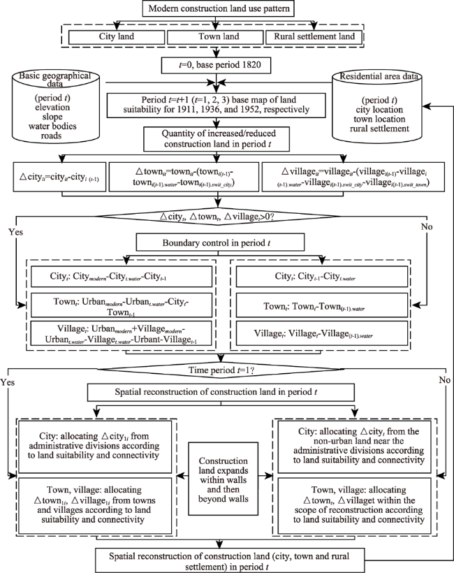
Figure 4 shows the detailed technical process.
Figure 4 Spatial reconstruction of historical construction land |
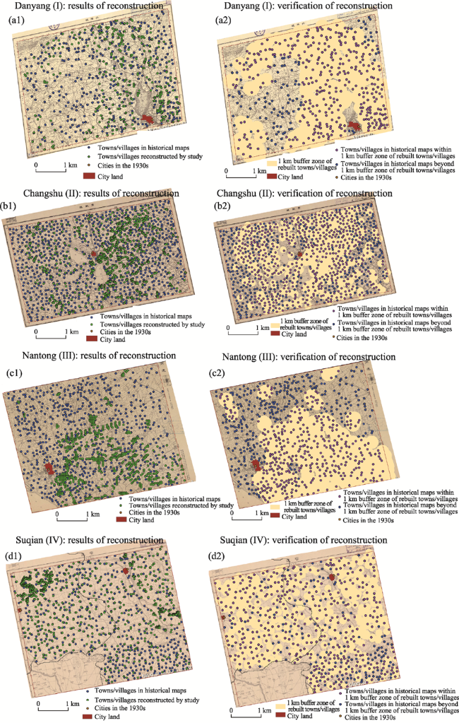
4.2.3 Reconstruction results
For the year 1820, the urban construction land and rural settlement land are defined by the number of grids corresponding to the estimated quantity while shapes of city/town walls are used as control borders. The suitability and connectivity of grids are also been considered (
Lin et al., 2015).
As for the years 1911, 1936 and 1952, the urban construction land and rural settlement land are assumed to expand only within the scope of corresponding city/town/village at contemporary time. The city land expanded within walls and then beyond the walls according to the suitability and connectivity characteristics. The result of the land suitability evaluation has been deemed as a controlling parameter.
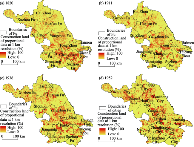
In order to improve the visual effect, the Boolean data in 200 m × 200 m grids has been converted into proportional data in 1 km × 1 km grids in
Figure 5. As shown in
Figure 5, the total construction land in Jiangsu has generally increased over the study period. However, there are significant differences across regions and periods. The spatial distribution of construction land exhibits its proclivity to water bodies and road networks and the great polarization effect of existent residence. Specifically, the construction land in 1820, 1911, 1936 and 1952 is shown below.
Figure 5 Spatial pattern of historical construction land in Jiangsu Province |
The construction land was distributed mainly in southern Jiangsu, about 53% of it is in Jiangning, Zhenjiang, Changzhou, Suzhou and Taicang.
It is straightforward that water bodies were of a great effect on the spatial pattern of the construction land. Rural settlements in central Jiangsu were mainly located at the junction of the main tributaries and along rivers/lakes to meet human production and living needs.
The densest distribution of rural settlements occurred in Zhenjiang, Changzhou, and the central and northern Suzhou from the south of the Yangtze River to Taihu Lake. The second densest area was found in western and southwestern Yangzhou along the Gaoyou Lake, western Tongzhou along the north of the Yangtze River, northwestern Huai’an along the downstream area of the Yellow River in northern Jiangsu Province.
The density of construction land in southern Jiangsu decreased rapidly because of the civil war. The total construction land slightly increased in central Jiangsu, and Huai’an, Xuzhou and Haizhou in northern Jiangsu. The construction land distribution density slightly increased in central Huai’an in northern Jiangsu and southwestern Xuzhou.
The construction land was densely distributed in western Tongzhou, central Yangzhou in central Jiangsu, and southeastern Xuzhou along the Luoma Lake, southern Haizhou along the Guanhe River, central and northern Huai’an, and southwestern Sizhou in northern Jiangsu. At the time, the total construction land rapidly increased with the construction of roads and railroads.
The construction land continued to increase. In particular, the construction land density rapidly increased in the coastal areas of Nantong.
In contrast, the construction land in central and southern Huai’an slightly decreased probably because of the reduction of water bodies.
