Orginal Article

Quality control and homogenization of daily meteorological data in the trans-boundary region of the Jhelum River basin

  • Rashid MAHMOOD ,
  • JIA Shaofeng
Expand
  • Key Laboratory of Water Cycle and Related Land Surface Processes, Institute of Geographic Science and Natural Resources Research, CAS, Beijing 100101, China

Author: Rashid Mahmood, E-mail: rashi1254@gmail.com; Jia Shaofeng, E-mail:

Received date: 2015-07-22

  Accepted date: 2015-10-29

  Online published: 2016-12-20

Supported by

National Natural Sciences Foundation of China, No.41471463

President’s International Fellowship Initiative CAS

Copyright

Journal of Geographical Sciences, All Rights Reserved

Abstract

Many studies such as climate variability, climate change, trend analysis, hydrological designs, agriculture decision-making etc. require long-term homogeneous datasets. Since homogeneous climate data is not available for climate analysis in Pakistan and India, the present study emphases on an extensive quality control and homogenization of daily maximum temperature, minimum temperature and precipitation data in the Jhelum River basin, Pakistan and India. A combination of different quality control methods and relative homogeneity tests were applied to achieve the objective of the study. To check the improvement after homogenization, correlation coefficients between the test and reference series calculated before and after the homogenization process were compared with each other. It was found that about 0.59%, 0.78% and 0.023% of the total data values are detected as outliers in maximum temperature, minimum temperature and precipitation data, respectively. About 32% of maximum temperature, 50% of minimum temperature and 7% of precipitation time series were inhomogeneous, in the Jhelum River basin. After the quality control and homogenization, 1% to 11% improvement was observed in the infected climate variables. This study concludes that precipitation daily time series are fairly homogeneous, except two stations (Naran and Gulmarg), and of a good quality. However, maximum and minimum temperature datasets require an extensive quality control and homogeneity check before using them into climate analysis in the Jhelum River basin.

Cite this article

Rashid MAHMOOD , JIA Shaofeng . Quality control and homogenization of daily meteorological data in the trans-boundary region of the Jhelum River basin[J]. Journal of Geographical Sciences, 2016 , 26(12) : 1661 -1674 . DOI: 10.1007/s11442-016-1351-7

1 Introduction

High quality and homogeneous long-term data series are essential in climate research, especially in climate change studies, which are used to assess climate variability and historical climate trends of mean and extreme climate events. However, most of the long climatic series not only have outliers and missing values but also are inhomogeneous (Cao and Yan, 2012; Trewin, 2013). Homogeneous climate time series are those where the variations are caused solely due to variation in climate and not due to non-climatic factors. The potential non-climatic factors are changes in instruments, changes in surroundings, relocation of monitoring stations, changes in observation methods etc. (Li-Juan and Zhong-Wei, 2012; Štěpánek et al., 2013). These factors may hide true signals of climate variability and climate change, leading towards some wrong conclusions of climate and hydrological studies (Costa and Soares, 2009). These are discussed in more details in Peterson et al. (1998), Aguilar et al. (2003) and Trewin (2010).
The climatic series that span from decades to centuries are rarely free of irregularities, errors and missing values. Although some specific inhomogeneous sites have only a marginal effect on the observed climate trends at the global scale, they can have substantial impact at the local or regional scale (Trewin, 2013). Thus, it is essential to produce homogeneous and quality controlled climate records before using them in climate analysis (Costa and Soares, 2009).
Several techniques such as Buishand range test (Buishand, 1982), Krukal-Wallis test (Kruskal, 1952; Kruskal and Wallis, 1952), Mann-Kendal test (Mann, 1945; Kendall, 1975), Multiple Analysis of Series for Homogenization (MASH) (Szentimrey, 1999), Pettit test (Pettitt, 1979), Regression-Based methods (Easterling and Peterson, 1995; Vincent, 1998), Standard Normal Homogeneity Test (SNHT) (Alexandersson, 1986) etc. have been developed for detection of irregularities on a site and their adjustment.
There are two main groups of homogeneity testing techniques; ‘absolute’ and ‘relative’. In the first group, the statistical tests are applied on each time series separately. In the relative methods, the statistical tests are applied on the difference of test series (time series under consideration) and reference series—created from some highly correlated stations in the region. Although both approaches are useful and valid to detect an inhomogeneity, the relative approach is more reliable than the absolute because it also considers the changes on the neighbor stations in the region (Peterson et al., 1998).
In homogenization, first, inhomogeneities are identified in a time series by using some techniques and then these irregularities are adjusted to make the site homogeneous (Trewin, 2013). Although several techniques are available, no single procedure is recommended.
Thus, the following four steps are commonly used to detect and adjust an inhomogeneous site: 1) basic quality control and metadata analysis, 2) reference series creation, 3) inhomogeneity detection and 4) adjustment for the compensation of inhomogeneity (Costa and Soares, 2009).
Many countries such as Australia (Trewin, 2013), Spain (Vicente-Serrano et al., 2010), Croatia (Zahradníček et al., 2014), Czech Republic (Štěpánek et al., 2009) and China (Feng et al., 2004) have developed homogenized meteorological datasets for climate analysis. However, in Pakistan and India, no quality controlled and homogeneous datasets are available for climate research. Thus, in the present study, quality controlled and homogeneous daily maximum temperature, minimum temperature and precipitation datasets are developed for the Jhelum River basin, Pakistan and India. This will provide an unprecedented resource for climate and climate change research in Pakistan. Station characteristics and data sources are described in Section 2. In Section 3, quality control and homogenization techniques are outlined. The main results and discussion are described in Section 4 and conclusions in Section 5.

2 Study area and data description

The upper Jhelum River basin is located in the north of Pakistan and spans between 33°-35°N and 73°-75.62°E, as shown in Figure 1. This is the second biggest tributary of the Indus River basin. The Jhelum basin has a drainage area of 33,342 km2, with an elevation ranging from 200 to 6248 m. The whole basin drains into the Mangla Reservoir, the second largest reservoir in Pakistan, which was construction in 1967. The primary function of this reservoir is to provide water for irrigation of 6 million ha of land and to produce electricity as byproduct. The installed capacity of the reservoir is 1000 MW, which is 6% of the installed capacity of the country’s power production (Archer and Fowler, 2008; Mahmood and Babel, 2013).
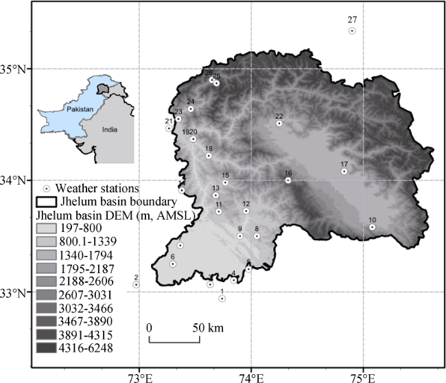
Figure 1 Location of the study area and geographic distribution of weather stations
Observed daily historical data of maximum temperature (22 weather stations), minimum temperature (22) and precipitation (27) were collected from Pakistan Meteorological Department (PMD), the Water and Power Development Authority of Pakistan (WAPDA) and the Indian Meteorological Department (IMD). The daily data of Gulmarg, Kupwara, Qazigund and Srinagar weather stations were obtained from IMD. The PMD provided climate data of Astore, Balakot, Garidopatta, Kotli, Muzaffarabad, Murree and Jhelum climate stations, and the remaining data was collected from WAPDA. Most of the precipitation series have data periods from 1961‒2009. However, most of the temperature time series range from 1971‒2009. The geographic distribution of these stations is shown in Figure 1. This shows that most of the stations are located in the eastern parts of the basin and on lower altitudes. The basic information about the stations such as location, mean distance between the stations, mean altitudinal differences between the stations, available data period and missing data of each station are given in Table 1.
Table 1 Geographic and basic information about the climate stations available in the Jhelum River basin

3 Methodology

3.1 Quality control

It is the primary emphasis of quality control to treat with outliers before application of any homogenization approach, which can mislead homogenization results (González-Rouco et al., 2001; Štěpánek et al., 2013; Zahradníček et al., 2014). There is a lack of generally recommended methodology for quality control of meteorological data. Thus, in the present study, a combination of different methods applied in Feng et al. (2004), Štěpánek et al. (2013) and Zahradníček et al. (2014) was used to identify erroneous data resulting from observation sources and digitization.
3.1.1 Extreme value check
In this method, daily values of a variable such as temperature are compared with the global and/or local historically observed extreme values of this variable. The data values which are greater than the highest and less than the lowest observed values of a variable are considered as erroneous values. These values are adjusted or removed from the data for subsequent quality control (Feng et al., 2004). In the present study, local temperature and precipitation extremes (PMD, 2014; Atta Ur and Shaw, 2015) were compared with the daily records to check outliers in the data series. These local extreme values for temperature and precipitation are presented in Table 2.
Table 2 Local extremes of Tx, Tn and Pr
Variable High Extreme Low Extreme Source
Tx (°C) 53.5 -24.1 (PMD, 2014; Atta Ur and Shaw, 2015)
Tn (°C) 53.5 -24.1
Pr (mm) 668 - (PMD, 2014)
3.1.2 Internal consistency check
Reek et al. (1992) concluded that the errors in the data series are mostly due to digitizing, unit difference, typos, different way of data reporting etc. So, they developed eight rules to check the erroneous data in meteorological time series. In the present study, the following three rules were used to check the daily time series, as used in Feng et al. (2004): 1) internal consistency detects the errors such as Tx is lower than Tn, 2) Flat-liner check recognizes the same data values for at least seven consecutive days (not applied to zero values of Pr) and 3) excessive diurnal temperature range (Tx-Tn>53.5°) is used to detect extraordinary large daily temperature range (Tx-Tn). Since no highest diurnal temperature range is found in the literature for Pakistan, a value of 53.5°—the highest maximum temperature in Pakistan—was used as the highest diurnal temperature range in the present study. If data values exceed the range of 53.5°, the values are identified as outliers.
3.1.3 Temporal outlier check
The above methods can detect some obvious errors in the data series. However, they cannot identify the errors such as where a data value is significantly different from the previous or the following value in the same time series (Feng et al., 2004). To detect these kinds of outliers, Tukey’s method, known as Inter Quartile Range (IQR) method, developed by Tukey (1997) was used in the present study, as in González-Rouco et al., (2001), Štěpánek et al. (2013) and Zahradníček et al. (2014) to detect the outliers in the climatic datasets. There are three main steps to detect outliers: 1) to find out the inter quartile range (IQR)—which is the difference between the first quartile (Q1) and the third quartile (Q3); 2) to calculate lower and upper extremes—the lower and upper extremes are calculated by subtracting 1.5×IQR from Q1 and adding 1.5×IQR into Q3, respectively; 3) values beyond these limits are considered to be possible outliers. If an IQR-coefficient of 3 is used, instead of 1.5, to calculate the upper and lower limits, then the values beyond these limits are considered to be the most probable outliers. This method is less sensitive to extreme values than the methods such as Z-score and Standard deviation method which use mean and/or standard deviation to detect outliers. This method has more resistant against outliers because quartiles are used in this method (Tukey, 1977; González-Rouco et al., 2001; Seo, 2006). In the present study, this method was applied on the differences of the test (specific station) and reference series (discussed in the next section) for the detection of erroneous data. In this study, IQR coefficient of 2 was used to give more assurance about outliers.
3.1.4 Spatial outlier check
This method is used to detect those outliers which are not detected by the previously mentioned methods. This method detects outliers by comparing test station values with neighbor stations’ values (Feng et al., 2004). Since no single method is generally recommended to deal with spatial outliers (Štěpánek et al., 2013), a combination of several methods was applied in the present study to identify outliers as done in Štěpánek et al. (2013) and Zahradníček et al. (2014). In this study, ProclimDB software developed by Štěpánek et al. (2010) was used for this purpose. This is a fully automated software for quality control of climate data. In this, several methods are available to detect spatial outliers. Among them, the following methods were used in the present study:
1) Pairwise comparison method. In this method, series of differences between test and neighbor stations are created and standardized. Cumulative density funtions (CDFs) for each difference series is calculated. If the average CDF exceeds the critical value (0.95), that value is considered as outlier. It means if the difference between the values at test and neighbor stations is statistically siginificant (α=0.05), the values of the test stations are considered as outliers.
2) Inter quartile range method. In this method, limits (higher and lower) are calculated from the neighbor stations and applied to the test series to find out the outliers. In the present study, a value of 2 (Tukey’s coefficient) was used during calculation of limits.
3) Technical series method. A technical (theoretical) series is created from neighbor stations by means of some statistical methods for spatial data (e.g., kriging and IDW). Then, this series is compared with the test series at a significance level of 0.5.
In the present study, five highly correlated neighbor stations, as discussed below, were used to create theoretical (technical) series for calculating limits for IQR method and for pairwise comparison method.
3.1.5 Creation of reference series
A change in a climatic time series which may be considered as an inhomogeneity in a dataset, but it may also be a result of a change in local or regional climate (Peterson et al., 1998). Several techniques have been introduced to overcome this kind of problems. Most of them use data from some highly correlated nearby stations in the region to establish a new time series (called as reference series) as a descriptor of regional climate. In the present study, a technique used in Zahradníček et al. (2014) and Štěpánek et al. (2013) was used to create reference series for each variable on each site. According to them, the first step is to select neighbour stations. These stations can be selected either by distances or by correlations. Correlation coefficients can be calculated either from raw station data or first order differences. In the present study, five highly correlated neighbor stations were selected, with the distance restricted to 150 km and altitude difference of 600 m. Then, the datasets of these highly correlated stations were standardized with the mean and standard deviation. At the end, Inverse Distance Weighting (IWD) method, equation 1, was used to take average of five selected standardized neighbors to create reference series.
where 
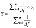
is the reference series; yi neighbor station; d is the distance between the test and neighbor stations; n is the number of neighbor stations; p is the power of distance—the higher the value of p, the greater the weights for the nearest neighbor station. In this study, a power of 0.5 and 1, as recommended in the manual of ProclimDB (Processing of Climatological Database) software (Štěpánek, 2010), was used to create reference series for temperature (Tx and Tn) and precipitation, respectively.

3.2 Homogenization

The presence of inhomogeneities is a common problem in climate time series. Most of these are related to abrupt changes in average values but also appears as changes in the trend of time series. These irregularities in climate data can deceive the actual results and lead to some wrong conclusions (Vicente-Serrano et al., 2010). Thus, to assess some meaningful climate analysis, the climate data must be homogeneous (Štěpánek et al., 2009). An ideal way to deal with such irregularities is to examine the station’s metadata—that records the historical information about station such as relocation of station, instrument change, type of instruments used etc. After detection of inhomogeneity through the metadata, the temporal variation of the inhomogeneous dataset from the station can be compared with the variation of the neighbor station or regional climate variation. However, most of the time, a complete metadata is not available for all stations in the region. Thus, some alternative subjective and objective methods are used to check the homogeneity (Feng et al., 2004). These methods are reviewed comprehensively in Peterson et al. (1998) and Costa and Soares (2009). These methods generally used the following steps during homogenization: 1) creation of reference series for comparison with the test series for relative homogenization, 2) application of statistical test to detect irregularities and 3) homogenization—adjustments to compensate with inhomogeneities and imputation of missing data. Since each statistical test renders results with some degree of uncertainty because of noise in the time series (Zahradníček et al., 2014), a combination of different tests is considered to be more effective to uncover data inhomogeneity. Thus, in this study, three relative homogeneity tests were applied for homogeneity check: SNHT (Alexandersson, 1986), Maronna and Yohai Bivariate test (Maronna and Yohai, 1978; Potter, 1981) and Easterling & Peterson test (Easterling and Peterson, 1995). Reference series for each test station were created from five highly correlated neighbor stations. These series can be divided into a duration of 40 years, with an overlap of 10 years if the series are of long period, e.g., more than 70 years. This is recommended for SNHT test to perform properly. Since there is a lack of methods to detect the inhomogeneities directly from the daily time series (Vicente-Serrano et al., 2010), these tests were applied on the monthly, seasonal and annual time series, the same as in Feng et al. (2004), Vicente-Serrano et al. (2010), Zahradníček et al. (2014) and Štěpánek et al. (2013). This approach is commonly used for inhomogeneity detection.
In ProclimDB, the main criterion for the identification of a year of breakpoint (abrupt change) is the probability of detection (PD) of a given year. This is the ratio of total detected breakpoints for a given year from all tests to the all theoretically possible breakpoints from all tests. PD values exceeding 10% and 20% (recommended by Štěpánek et al., 2010) are used to identify potential inhomogeneities in precipitation and temperature, respectively. The same values were used for the present study. Before taking the final decision about breakpoints, these breakpoints were also examined graphically to reduce any uncertainty.
The inhomogeneous series were corrected on a daily scale. The daily adjustments were calculated based on the reference series and smoothed by low pass filter because this better reflects the physical properties of time series (Figure 1). A 15-year data on both sides of breakpoint was used during the calculation of adjustments.
In adjustment calculation, first the difference series between the test and reference series are calculated before and after the breakpoint. Then, the adjustments are calculated by subtracting the difference series before breakpoint and the difference series after breakpoint. These adjustments can be smoothed by low pass filter, high pass filter or moving average (Štěpánek et al., 2013).
For validation of homogenization, correlation coefficients between test and reference series are calculated for each month before application of adjustments and after application of adjustments. Then, these correlations are compared with each other. If there is an increase in change in correlation coefficients, the adjustments are accepted (Zahradníček et al., 2014). The same was done in the present study.
The presence of missing data in climate time series is a common problem which must be considered when dealing statistically with the climate data. It can mislead the results and even prevent important analysis of the considered variable from being carried out. Currently, several statistical techniques have been developed to overcome this problem. They span from some simple methods, such as using a mean value, to some very sophisticated techniques, such as multiple imputation. However, their application depends mainly on the percentage of missing data. It is suggested that if percentage of missing values is not greater than 5, any method can be used. However, if percentage of missing values is greater than 5, some sophisticated methods such as regression and multiple imputation methods must be applied (Lo Presti et al., 2010). In the present study, a multiple imputation method, predictive mean matching (Heitjan and Little, 1991), was used to deal with missing data because most of the stations available for this study have missing data greater than 5%. On some stations, the missing percentage is even greater than 15% (Table 1). This is a semi-parametric approach which is similar to regression method except that these missing values are imputed randomly. This method ensures that the imputed values are plausible. It may perform better than regression if the normality assumption is violated (Horton and Lipsitz, 2001).

4 Results and discussion

4.1 Spatial correlation

For homogenization and quality control of climate data, it is essential to get information about spatial correlations among climate stations. Figure 2 shows average correlation coefficient of each climate station with all the other stations in the study area. The correlations were calculated for each variable (Tx, Tn and Pr) between stations, on daily time series. In case of Tx, the highest correlation (0.95) was observed on Kallar, Kotli, Muzaffarabad and Srinagar and the lowest (0.79) on Bagh. In case of Tn, the highest correlation (0.96) was found on Mangla, Srinagar, Domel and Muzaffarabad and the lowest (0.85) on Dhudial. Among Pr stations, Domel had the highest correlation of 0.62, and Gulmarg had the lowest correlation of 0.2. The spatial correlations for Tx and Tn were much stronger than Pr.
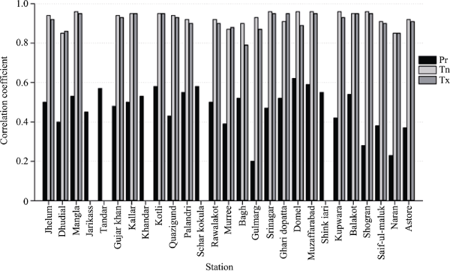
Figure 2 Average correlation coefficients between weather stations in the Jhelum River basin
Figure 3 shows average correlations with respect to distance between climate stations in case of Tx, Tn and Pr. Highly correlated stations were observed within 40 km. As distance exceeded 40 km, correlations decreased quickly in case of Pr. On the other hand, in case of temperature, decreasing rate was very small. As expected, larger distances showed lower correlations between stations. As distance increased, the correlations decreased more quickly in precipitation as compared to temperature.
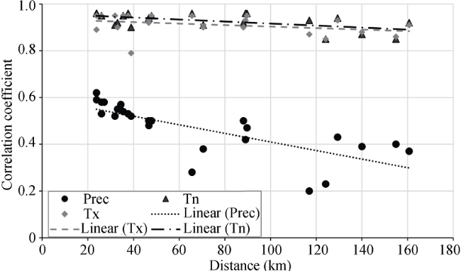
Figure 3 Variation in correlation coefficients with respect to distance between weather stations in the Jhelum River basin

4.2 Quality control of daily data

In the present study, an extensive methodology comprising four checks (high/low extremes,internal consistency, temporal, and spatial outliers’ checks) were used to detect outliers. Table 3 shows percentage of outliers detected by each quality control method in Tx, Tn and Pr. These are the total outliers detected on all climate stations, in three variables (Tx, Tn and Pr). Very few values 6 (0.0019%), 24 (0.0076%) and 4 (0.001%) were identified by high/low extreme check in Tx, Tn and Pr, respectively. These values were adjusted manually by examining the neighbor station values as well as previous and following values around the infected value. A total of 846 (0.211%) were recognized as errors in Tx and Tn time series during the internal constancy check. Among them, 354 (0.0558%) errors were identified by Tx lower than Tn rule, and no error was detected by excessive diurnal range check. These errors were corrected by taking the average of five neighbor stations, and previous and following values of the infected value. Flat-liner check (same seven consecutive values) detected about 216 (0.0677%) values in Tx and 276 (0.0874%) in Tn time series. In this case, all values were removed from the datasets except the first value of each group of same consecutive values, the same as in Feng et al. (2004).
Table 3 Percentages of erroneous data in Tx, Tn and Pr time series during quality control in the Jhelum River basin
Method Tx (%) Tn (%) Pr (%)
Total number of values processed 319100 315794 418499
High/Low extremes 0.0019 0.0076 0.0010
Internal consistency Tx lower than Tn 0.0279 0.0279
Flat-liner 0.0677 0.0874 0.0000
Excessive diurnal temperature range 0.0000 0.0000
Temporal outliers 0.2407 0.2825
Spatial outliers 0.2288 0.3467 0.0222
Total 0.5669 0.7521 0.0232
Tukey’s method detected 768 (0.241%) and 892 (0.283%) temporal outliers in Tx and Tn, respectively, and 730 (0.229%) and 1095 (0.347%) errors were identified by spatial outliers method. The errors detected by temporal and spatial outliers check were removed from the datasets before homogenization process. Table 3 shows that the most infected variable is Tn, and the less effected variable is Pr. Since, according to the best of our knowledge, no studies are reported on quality control in the Jhelum basin, these results were compared with Feng et al. (2004) conducted in China. It was found that Tx and Tn are more problematic than Chinese stations. Nonetheless, precipitation data is of high quality, which is comparable with China precipitation data.

4.3 Homogenization

Table 4 describes the number of stations having inhomogeneous datasets, the number of inhomogeneities in climate variables, and the years of inhomogeneities. A total of 23 inhomogeneities (2 in Pr time series, 9 in Tx, and 12 in Tn) and datasets of 20 stations (2 in Pr time series, 7 in Tx, and 11 in Tn) were identified as inhomogeneous. This means 28% of the climatic series (Tx, Tn and Pr) were found as inhomogeneous. Most of the inhomogeneous stations were found in Tx and Tn data series, with 7 (32%) and 11 (50%) stations, respectively. Only 2 (7%) of the Pr data series were detected as inhomogeneous. Some example of inhomogeneous station and breakpoints detected are show in Figure 4. Since no studies about homogenization are found in Pakistan, these results were compared with some other studies such as Feng et al. (2004) conducted in China, Štěpánek et al. (2013) in Czech Republic and Zahradníček et al. (2014) in Croatia. In Feng et al. (2004), Štěpánek et al. (2013) and Zahradníček et al. (2014), a percentage of inhomogeous stations was 37%, 42% and 23%, respectively. However, they conducted homogenization on more climate variables than this study.
Table 4 Inhomogeneous stations and number of breakpoints in Tx, Tn and Pr in the Jhelum River basin
SR Station Year of inhomogeneities
Tx Tn Pr
1 Bagh 1970 1970, 2004
2 Balakot 1979
3 Dhudial 1989 1989
4 Domel 1969, 1989 1969
5 Gulmarg 1987 1968
6 Gharidopatta 1969
7 Kotli 1981, 1995 1970
8 Kupwara 1985
9 Mangla 1972
10 Murree 1989 1989
11 Muzaffarabad 1969 1969
12 Naran 1989 1988
13 Rawalakot 1990
Stations having inhomogeneities 7 11 2
Stations having inhomogeneities (%) 31.8 50.0 7.4
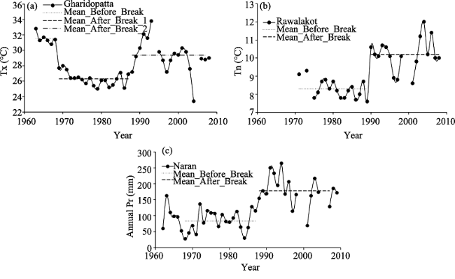
Figure 4 Detected inhomogeneities (a) in Tx on Gharidopatta weather station, (b) in Tn on Rawalakot and (c) in Pr on Naran, in the Jhelum River basin
When some data series are detected as inhomogeneous, that data then become questionable or invalid for climate change, climate variability and trend analysis (Feng et al., 2004). Since overall 28% of the stations are inhomogeneous, it is necessary to remove inhomoge-neities from data series to make it useful for climate analysis in the Jhelum River basin. So,correction (adjustments) were calculated for each inhomogeneous climate station from daily reference series and then adjusted with the infected raw data to compensate the breakpoints. An example of adjustments calculated for the breakpoint in 1990 for Tn of Rawalakot station is shown in Figure 5.
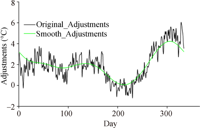
Figure 5 Daily adjustments for the identified breakpoint in 1990 in Tn of Rawalakot station (shown in Figure 4b)
Figure 6 shows changes in average correlation coefficients (CC) calculated between the test and reference series before and after homogenization, on the infected climate stations. These changes were calculated for each climate station and for each climate variable (Tx, Tn and Pr), and then the monthly average change in CC was taken for all infected climate station. Increasing (positive) change in CC means improvement after homogenization, and decreasing (negative) change means no improvement in data series. Almost all months showed positive change except September (in case of Pr), October (Tx), and November (Pr). The improvement is ranged from 2% to 11% in Tx, from 1% to 8% in Tn and 0.1% to 3% in case of Pr, as shown in Figure 6. The maximum improvement was observed in the month of March (in case of Tx), August (Tn) and March (Pr). On the whole, after homogenization, the climate time series are improved and can be used for further climate analysis.
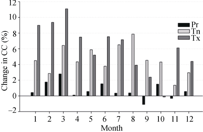
Figure 6 Change in correlation coefficients (CC) between test and reference series before and after homogenization

5 Conclusions

In the present study, daily climate data (maximum temperature, minimum temperature and precipitation) of the Jhelum River basin was extensively quality controlled by applying a combination of different methods (high/low extreme check, internal consistency check, temporal and spatial outlier check). Then, inhomogeneities were detected by a combination of relative homogeneity methods (Standard Normal Homogeneity Test (SNHT), Bivariate test and Easterling & Peterson test) and adjusted by applying correction factors calculated from the reference series on daily basis.
During quality control, 0.59%, 0.78% and 0.023% of the total data values were detected as outliers in maximum temperature, minimum temperature and precipitation time series, respectively. During homogenization, maximum temperature series of 32%, minimum temperature series of 50% and precipitation series of 7% were identified as inhomogeneous, in the Jhelum River basin. After homogenization, the infected series were improved by 1% to 11%.
It was concluded that the precipitation daily time series are fairly homogeneous, except two stations (Naran and Gulmarg), and of a good quality. However, the maximum and minimum temperature datasets require an extensive quality control and homogeneity check before using them in climate analysis, especially in climate variability, climate change and trend analysis. The homogenized dataset will be used to assess the impact of climate change on the water resources of the Jhelum River basin in further studies.

The authors have declared that no competing interests exist.

1
Aguilar E, Auer I, Brunet M et al., 2003. Guidelines on Climate Metadata and Homogenization WMO/TD No.1186. W. M. Organization: Geneva, 52 pp.

2
Alexandersson H, 1986. A homogeneity test applied to precipitation data.Journal of Climatology, 6: 661-675. doi: 10.1002/joc.3370060607.Abstract In climate research it is important to have access to reliable data which are free from artificial trends or changes. One way of checking the reliability of a climate series is to compare it with surrounding stations. This is the idea behind all tests of the relative homogeneity. Here we will present a simple homogeneity test and apply it to a precipitation data set from south-western Sweden. More precisely we will apply it to ratios between station values and some reference values. The reference value is a form of a mean value from surrounding stations. It is found valuable to include short and incomplete series in the reference value. The test can be used as an instrument for quality control as far as the mean level of, for instance, precipitation is concerned. In practice it should be used along with the available station history. Several non-homogeneities are present in these series and probably reflect a serious source of uncertainty in studies of climatic trends and climatic change all over the world. The significant breaks varied from 5 to 25 per cent for this data set. An example illustrates the importance of using relevant climatic normals that refer to the present measurement conditions in constructing maps of anomalies.

DOI

3
Archer D R, Fowler H J, .

4
Atta Ur R, Shaw R, 2015. Disaster and climate change education in Pakistan. In: Rahman A U, Khan A N, Shaw R (eds.) Disaster Risk Reduction Approaches in Pakistan. Japan: Springer, 315-335.Pakistan is vulnerable to wide range of hazards and rooting from weather, hydrological, geophysical and human induced disasters. In the past three decades, there has been an increase in the frequency and intensity of hydro-meteorological disasters including floods, extreme temperatures, torrential and prolonged rainfall, drought and storms. In this regard, efforts have been made by the government to endorse disaster and climate change education, and so far variety of initiatives and activities have been planned and some of them implemented. Because, Hyogo Framework for Action (HFA) 2005 2015, priority for action-3 emphasises the role of knowledge and education, and stress on formal and non-formal education and awareness-raising as an important component of disaster risk reduction strategy. Keeping in view this changing scenario, the government of Pakistan has developed the national climate change policy 2012, which clearly pinpointed the need for disaster and climate change education and development of curricula with particular emphasis on disaster and climate change, and its introduction in the country education system. The policy also highlighted to ensure inclusion of climate change education and training as a compulsory subject in the forest education system. In order to enhance the human capacity in the field of disaster and climate change education, the government has also taken the responsibility of sending young scientists and students to reputed institutions abroad for higher studies. In addition to this, it is pertinent to encourage and strengthen the existing disaster and climate change science, in the related institutions and universities through technical and financial support. The national disaster management plan 2012 2022 also highlighted that research need to be carried out on the challenges of disasters and climate change issues. These measures if taken care of in policy, plans and programs will definitely lead to mitigate and minimize the extent of damages in anticipation to the changing climate scenario. This chapter discusses the disaster and climate change education, Pakistan vulnerability to Disaster and Climate Change, Growth and Development of Disaster Legislations and Institutions, Disaster and Climate Change Education at School, College, University, Professional and Technical Institutions, National Institute for Disaster Management, Religious Institutions, Community Level, and in the State Departments, Civil Services Academies and promotion of Research environment in the country.

DOI

5
Buishand T A, .

6
Cao L J, Yan Z W, 2012. Progress in research on homogenization of climate data.Adv. Clim. Change Res., 3: 59-67. doi: 10.3724/SP.J.1248.2012.00059.

DOI

7
Costa A, Soares A, 2009. Homogenization of climate data: Review and new perspectives using geostatistics.Math. Geosci., 41: 291-305. doi: 10.1007/s11004-008-9203-3.The homogenization of climate data is of major importance because non-climatic factors make data unrepresentative of the actual climate variation, and thus the conclusions of climatic and hydrological studies are potentially biased. A great deal of effort has been made in the last two decades to develop procedures to identify and remove non-climatic inhomogeneities. This paper reviews the characteristics of several widely used procedures and discusses the potential advantages of geostatistical techniques. In a case study, the geostatistical simulation approach is applied to precipitation data from 66 monitoring stations located in the southern region of Portugal (1980鈥2001). The results from this procedure are then compared with those from three well established statistical tests: the Standard normal homogeneity test (SNHT) for a single break, the Buishand range test, and the Pettit test. Promising results from the case study open new research perspectives on the homogenization of climate time series.

DOI

8
Easterling D R, Peterson T C, 1995. A new method for detecting undocumented discontinuities in climatological time series.International Journal of Climatology, 15: 369-377. doi: 10.1002/joc.3370150403.Abstract The development of homogeneous climatological time series is a crucial step in examining climate fluctuations and change. We review and test methods that have been proposed previously for detecting inhomogeneities, and introduce a new method we have developed. This method is based on a combination of regression analysis and non-parametric statistics. After evaluation against other techniques, using both simulated and observed data, our technique appears to have the best overall performance.

DOI

9
Feng S, Hu Q, Qian W, 2004. Quality control of daily meteorological data in China, 1951-2000: A new dataset.International Journal of Climatology, 24: 853-870. doi: 10.1002/joc.1047.Abstract Long-term observational data are essential for understanding local and regional climate and climate change. These data are also important for hydrological designs and agricultural decision making. This study examined the daily meteorological data from 726 stations in China from 1951 to 2000, and developed an unprecedented climatic dataset that contains 10 daily variables: maximum and minimum surface air temperatures, mean surface air temperature, skin surface temperature, surface air relative humidity, wind speed, wind gust, sunshine duration hours, precipitation, and pan evaporation. The characteristics of the original stations' data and quality-control methods designed and used in developing this dataset are detailed. The quality-control procedures identified less than 0.05% of the data records as being erroneous because of typos and incorrect units, reading, or data coding. When the spatial and temporal consistency of the variables' time series were inspected, nearly 37.9% of the stations were found to have one or more variables with inconsistent changes. The sources causing the temporal inconsistency/discontinuity were evaluated, and a method was developed and applied to adjust those data segments containing inconsistent values. The resulting data series, as an alternative to the original quality-controlled series, showed both spatially and temporally consistent trends in the occurrence frequency of extreme climate events compared with the unadjusted data series. Finally, the quality-controlled daily data were gridded to a 1.0 1.0 grid system covering China after the erroneous and missing data were estimated. This new dataset opens up opportunities for analysing and understanding the climate variability and climate change in China. Copyright 2004 Royal Meteorological Society

DOI

10
González-Rouco J F, Jiménez J L, Quesada V et al., 2001. Quality control and homogeneity of precipitation data in the southwest of Europe. Journal of Climate, 14: 964–978. doi: 10.1175/1520-0442(2001)014 <0964: QCAHOP >2.0.CO; 2.A quality control process involving outliers processing, homogenization, and interpolation has been applied to 95 monthly precipitation series in the Iberian Peninsula, southern France, and northern Africa during the period 1899-1989. A detailed description of the procedure results is provided and the impact of adjustments on trend estimation is discussed.Outliers have been censored by trimming extreme values. Homogeneity adjustments have been developed by applying the Standard Normal Homogeneity Test in combination with an objective methodology to select reference series.The spatial distribution of outliers indicates that they are due to climate variability rather than measurement errors. After carrying out the homogeneity procedure, 40% of the series were found to be homogeneous, 49.5% became homogeneous after one adjustment, and 9.5% after two adjustments. About 30% of the inhomogeneities could be traced to information in the scarce history files.It is shown that these data present severe homogeneity problems and that applying outliers and homogeneity adjustments greatly changes the patterns of trends for this area.

DOI

11
Heitjan D, Little R, 1991. Multiple imputation for the fatal accident reporting system.Journal of the Royal Statistical Society. Series C (Applied Statistics), 40: 13-29. doi: 10.2307/2347902.The Fatal Accident Reporting System (FARS) is a database collected for the US National Highway Traffic Safety Administration (NHTSA) at the site of all fatal traffic accidents. Variables include location and time of accident, number and position of vehicles, age, sex and driving record of the driver, seat-belt use and blood alcohol content of the driver. The last two variables are of great interest but have substantial proportions of missing data. The NHTSA is interested in a method of imputation that allows appropriate estimates and standard errors to be computed from the filled-in data. This paper explores the use of multiple imputation based on predictive mean matching as a means of achieving these goals. Two specific methods are described and applied to a sample of the FARS data. A simulation study compares the frequency properties of the methods.

DOI

12
Horton N J, Lipsitz S R, 2001. Multiple imputation in practice: Comparison of software packages for regression models with missing variables.The American Statistician, 55: 244-254. doi: 10.2307/2685809.

DOI

13
Kendall M G, 1975. Rank Correlation Methods (Charles Griffin). London: Oxford University Press.

14
Kruskal W H, 1952. A nonparametric test for the several sample problem.The Annals of Mathematical Statistics, 23: 525-540. doi: 10.2307/2236578.Suppose that $C$ independent random samples of sizes $n_1, cdots, n_c$ are to be drawn from $C$ univariate populations with unknown cumulative distribution functions $F_1, cdots, F_c$. This paper discusses a test of the null hypothesis $F_1 = F_2 = cdots = F_c$ against alternatives of the form $F_i(x) = F(x - theta_i)quad (text{all} x, i = 1, cdots, C)$ with the $theta_i$'s not all equal, or against alternatives of a much more general sort to be specified in Section 5. The test to be discussed has as its critical region large values of the ordinary $F$-ratio for one-way analysis of variance, computed after the observations have been replaced by their ranks in the $sum n_i$-fold over-all sample. This use of ranks simplifies the distribution theory, and permits application of the test to cases where the ranks are available but the numerical values of the observations are difficult to obtain. Briefly, then, we shall consider a non-parametric analogue, based on ranks, of one-way analysis of variance. It is shown in Section 4 that, under quite general conditions, the proposed test statistic, $H$, is asymptotically chi-square with $C - 1$ degrees of freedom when the null hypothesis holds. Section 5 derives a necessary and sufficient condition that the natural family of sequences of tests based on large values of $H$ all be consistent against a given alternative. Section 6 derives the variance of $H$ under the null hypothesis, Section 7 derives the maximum value of $H$, and Section 8 gives a difference equation which may be used to obtain exact small-sample distributions under the null hypothesis. These derivations are made on the assumption of continuity for the cumulative distribution functions; Section 9 considers extensions to the possibly discontinuous case.

DOI

15
Kruskal W H, Wallis W A, 1952. Use of ranks in one-criterion variance analysis.Journal of the American Statistical Association, 47: 583-621. doi: 10.2307/2280779.ABSTRACT Given C samples, with ni observations in the ith sample, a test of the hypothesis that the samples are from the same population may be made by ranking the observations from from 1 to ni (giving each observation in a group of ties the mean of the ranks tied for), finding the C sums of ranks, and computing a statistic H. Under the stated hypothesis, H is distributed approximately as (C &ndash; 1), unless the samples are too small, in which case special approximations or exact tables are provided. One of the most important applications of the test is in detecting differences among the population means.** Based in part on research supported by the Office of Naval Research at the Statistical Research Center, University of Chicago.

DOI

16
Lo Presti R, Barca E, Passarella G, 2010. A methodology for treating missing data applied to daily rainfall data in the Candelaro River Basin (Italy).Environ. Monit. Assess., 160: 1-22. doi: 10.1007/s10661-008-0653-3.Environmental time series are often affected by the "presence" of missing data, but when dealing statistically with data, the need to fill in the gaps estimating the missing values must be considered. At present, a large number of statistical techniques are available to achieve this objective; they range from very simple methods, such as using the sample mean, to very sophisticated ones, such as multiple imputation. A brand new methodology for missing data estimation is proposed, which tries to merge the obvious advantages of the simplest techniques (e.g. their vocation to be easily implemented) with the strength of the newest techniques. The proposed method consists in the application of two consecutive stages: once it has been ascertained that a specific monitoring station is affected by missing data, the "most similar" monitoring stations are identified among neighbouring stations on the basis of a suitable similarity coefficient; in the second stage, a regressive method is applied in order to estimate the missing data. In this paper, four different regressive methods are applied and compared, in order to determine which is the most reliable for filling in the gaps, using rainfall data series measured in the Candelaro River Basin located in South Italy.

DOI PMID

17
Mahmood R, Babel M S, 2013. Evaluation of SDSM developed by annual and monthly sub-models for downscaling temperature and precipitation in the Jhelum basin, Pakistan and India.Theor. Appl. Climatol., 113: 27-44. doi: 10.1007/s00704-012-0765-0.The study evaluates statistical downscaling model (SDSM) developed by annual and monthly sub-models for downscaling maximum temperature, minimum temperature, and precipitation, and assesses future changes in climate in the Jhelum River basin, Pakistan and India. Additionally, bias correction is applied on downscaled climate variables. The mean explained variances of 66, 76, and 1102% for max temperature, min temperature, and precipitation, respectively, are obtained during calibration of SDSM with NCEP predictors, which are selected through a quantitative procedure. During validation, average R 2 values by the annual sub-model (SDSM-A)—followed by bias correction using NCEP, H3A2, and H3B2—lie between 98.4 and 99.102% for both max and min temperature, and 77 to 8502% for precipitation. As for the monthly sub-model (SDSM-M), followed by bias correction, average R 2 values lie between 98.5 and 99.502% for both max and min temperature and 75 to 8302% for precipitation. These results indicate a good applicability of SDSM-A and SDSM-M for downscaling max temperature, min temperature, and precipitation under H3A2 and H3B2 scenarios for future periods of the 2020s, 2050s, and 2080s in this basin. Both sub-models show a mean annual increase in max temperature, min temperature, and precipitation. Under H3A2, and according to both sub-models, changes in max temperature, min temperature, and precipitation are projected as 0.91–3.1502°C, 0.93–2.6302°C, and 6–1202%, and under H3B2, the values of change are 0.69–1.9202°C, 0.56–1.6302°C, and 8–1402% in 2020s, 2050s, and 2080s. These results show that the climate of the basin will be warmer and wetter relative to the baseline period. SDSM-A, most of the time, projects higher changes in climate than SDSM-M. It can also be concluded that although SDSM-A performed well in predicting mean annual values, it cannot be used with regard to monthly and seasonal variations, especially in the case of precipitation unless correction is applied.

DOI

18
Mann H B, 1945. Nonparametric tests against trend.Econometrica, 13: 245-259. doi: 10.2307/1907187.

19
Maronna R, Yohai V J, 1978. A bivariate test for the detection of a systematic change in mean.Journal of the American Statistical Association, 73: 640-645. doi: 10.2307/2286616.Ricardo Maronna is a Private Consultant Paraguay 1283 (2, 3), 1057 Buenos Aires, Argentina.

DOI

20
Peterson T C, Easterling D R, Karl T R et al., 1998. Homogeneity adjustments of in situ atmospheric climate data: A review. International Journal of Climatology, 18: 1493–1517. doi: 10.1002/(SICI)1097-0088(19981115) 18:13<1493::AID-JOC329>3.0.CO;2-T.Long-term in situ observations are widely used in a variety of climate analyses. Unfortunately, most decade- to century-scale time series of atmospheric data have been adversely impacted by inhomogeneities caused by, for example, changes in instrumentation, station moves, changes in the local environment such as urbanization, or the introduction of different observing practices like a new formula for calculating mean daily temperature or different observation times. If these inhomogeneities are not accounted for properly, the results of climate analyses using these data can be erroneous. Over the last decade, many climatologists have put a great deal of effort into developing techniques to identify inhomogeneities and adjust climatic time series to compensate for the biases produced by the inhomogeneities. It is important for users of homogeneity-adjusted data to understand how the data were adjusted and what impacts these adjustments are likely to make on their analyses. And it is important for developers of homogeneity-adjusted data sets to compare readily the different techniques most commonly used today. Therefore, this paper reviews the methods and techniques developed for homogeneity adjustments and describes many different approaches and philosophies involved in adjusting in situ climate data.

DOI

21
Pettitt A N, 1979. A non-parametric approach to the change-point problem.Applied Statistics, 28: 126-135. doi: 10.2307/2346729.Non-parametric techniques are introduced for the change-point problem. Exact and approximate results are obtained for testing the null hypothesis of no change. The methods are illustrated by the analysis of three sets of data illustrating the techniques for zero-one observations, Binomial observations and continuous observations. Some comparisons are made with methods based on CUSUMS. [ABSTRACT FROM AUTHOR]

DOI

22
PMD, cited 2015: Extreme Events Reports. [Available online at cited 2015.]

23
Potter K W, 1981. Illustration of a new test for detecting a shift in mean in precipitation series. Monthly Weather Review, 109: 2040–2045. doi: 10.1175/1520-0493(1981)109<2040:IOANTF>2.0.CO;2.

24
Seo S, 2006. A review and comparison of methods for detecting outliers in univariate data sets University of Pittsburgh 59 pp.Most real-world data sets contain outliers that have unusually large or small values when compared with others in the data set. Outliers may cause a negative effect on data analyses, such as ANOVA and regression, based on distribution assumptions, or may provide useful information about data when we look into an unusual response to a given study. Thus, outlier detection is an important part of data analysis in the above two cases. Several outlier labeling methods have been developed. Some methods are sensitive to extreme values, like the SD method, and others are resistant to extreme values, like Tukey's method. Although these methods are quite powerful with large normal data, it may be problematic to apply them to non-normal data or small sample sizes without knowledge of their characteristics in these circumstances. This is because each labeling method has different measures to detect outliers, and expected outlier percentages change differently according to the sample size or distribution type of the data. Many kinds of data regarding public health are often skewed, usually to the right, and lognormal distributions can often be applied to such skewed data, for instance, surgical procedure times, blood pressure, and assessment of toxic compounds in environmental analysis. This paper reviews and compares several common and less common outlier labeling methods and presents information that shows how the percent of outliers changes in each method according to the skewness and sample size of lognormal distributions through simulations and application to real data sets. These results may help establish guidelines for the choice of outlier detection methods in skewed data, which are often sen in the public health field.

25
Štěpánek P, cited 2015: ProClimDB - Software for Processing Climatological Datasets. Available online at cited 2015.

26
Štěpánek P, Zahradníček P, Skalák P, 2009. Data quality control and homogenization of air temperature and precipitation series in the area of the Czech Republic in the period 1961-2007.Advances in Science and Research, 3: 23-26. doi: 10.5194/asr-3-23-2009.

27
Štěpánek P, Zahradníček P, Farda A, 2013. Experiences with data quality control and homogenization of daily records of various meteorological elements in the Czech Republic in the period 1961-2010.Quarterly Journal of the Hungarian Meteorological Service, 117: 1-158.

28
Szentimrey T, 1999: Multiple analysis of series for homogenization (MASH). Proceedings of the Second Seminar for Homogenization of Surface Climatological Data, Budapest, Hungary, 27-46.

29
Trewin B, 2013. A daily homogenized temperature data set for Australia.International Journal of Climatology, 33: 1510-1529. doi: 10.1002/joc.3530.A new homogenized daily maximum and minimum temperature data set, the Australian Climate Observations Reference NetworkSurface Air Temperature data set, has been developed for Australia. This data set contains data from 112 locations across Australia, and extends from 1910 to the present, with 60 locations having data for the full post-1910 period. These data have been comprehensively analysed for inhomogeneities and data errors ensuring a set of station temperature data which are suitable for the analysis of climate variability and trends. For the purposes of merging station series and correcting inhomogeneities, the data set has been developed using a technique, the percentile-matching (PM) algorithm, which applies differing adjustments to daily data depending on their position in the frequency distribution. This method is intended to produce data sets that are homogeneous for higher-order statistical properties, such as variance and the frequency of extremes, as well as for mean values. The PM algorithm is evaluated and found to have clear advantages over adjustments based on monthly means, particularly in the homogenization of temperature extremes. Copyright (c) 2012 Royal Meteorological Society

DOI

30
Tukey J W, 1977. Exploratory Data Analysis. Pearson.

31
Vicente-Serrano S M, Beguería S, López-Moreno J I et al., 2010. A complete daily precipitation database for northeast Spain: Reconstruction, quality control, and homogeneity. International Journal of Climatology, 30: 1146–1163. doi: 10.1002/joc.1850.Abstract Top of page Abstract 1.Introduction 2.Database 3.Methodology 4.Results 5.Conclusions Acknowledgements References This paper reports the procedure used in creating a homogeneous database of daily precipitation in northeast Spain. The source database comprised 3106 daily precipitation observatories, with data ranging from 1901 to 2002. Firstly, a reconstruction of the series was performed. Data from adjacent observatories were combined to provide long temporal coverage. Data gaps were filled using values from the nearest neighbour observatories. A distance threshold was set to avoid the introduction of spurious information in the series. Secondly, the reconstructed series were subjected to a quality control process. Empirical percentiles corresponding to each precipitation observation were compared to the percentiles corresponding to the closest neighbour observatory, and a threshold difference was set to identify questionable extremes. After careful inspection of each case, 0.1% of the data was rejected and replaced with information from the nearest neighbour. Thirdly, the homogeneity of the series was checked using the standard normal homogeneity test. This allowed detection of inconsistencies present in the original database or introduced by the reconstruction process. Four parameters were assessed at a monthly level: amount of precipitation, number of rainy days, daily maxima, and number of days above the 99th percentile. A total of 43% of the series had some periods of inhomogeneity and were discarded. The final database comprised 828 series with varying time coverages. The greatest number of stations existed during the 1990s, but more than 300 series contained information from the 1960s, and 34 series contained a complete record since 1920. Comparisons of the spatial variability of several parameters describing the daily precipitation characteristics were made. The results showed that the final database had improved spatial coherence. The process described here is proposed as a model for developing a standard procedure for the construction of databases of daily climate data. Copyright 2010 Royal Meteorological Society

DOI

32
Vincent L A, 1998. A technique for the identification of inhomogeneities in Canadian temperature series. Journal of Climate, 11: 1094–1104. doi: 10.1175/1520-0442(1998)011<1094:ATFTIO>2.0.CO;2.A new technique has been developed for the identification of inhomogeneities in Canadian temperature series. The objective is to identify two types of inhomogeneities-nonclimatic steps and trends-in the series of a candidate station in the absence of prior knowledge of the time of site changes and to properly estimate their position in time and their magnitude. This new technique is based on the application of four linear regression models in order to determine whether the tested series is homogeneous, if there is a nonclimatic trend, a step, or trends before and/or after a step. The dependent variable is the series of the candidate station and the independent variables are the series of some neighboring stations. Additional independent variables are used to describe and measure steps and trends existing in the tested series but not in the neighboring series. After the application of each model, the residuals are analyzed in order to determine the fit of the model. If there is significant autocorrelation in the residuals, nonidentified inhomogeneities are suspected in the tested series and a different model is applied to the datasets. A model is finally accepted when the residuals are considered to be random variables. The description of the technique is presented along with some evaluation of its ability to identify inhomogeneities. Results are illustrated through the provision of an example of its application to archived temperature datasets.

DOI

33
Zahradníček P, Rasol D, Cindrić K et al., 2014. Homogenization of monthly precipitation time series in Croatia. International Journal of Climatology, 34: 3671–3682. doi: 10.1002/joc.3934.ABSTRACT Various types of studies require a sufficiently long series of data processed identically over the entire area. For climate analysis, it is necessary that analysed time series are homogeneous, which means that their variations are caused only by variations in weather and climate. Unfortunately, most of the climatological series are inhomogeneous and contain outliers that may significantly affect the analysis results. The 137 stations with precipitation measurement belonging to the meteorological station network governed by the Meteorological and Hydrological Service of Croatia were selected for the present analysis. Most of the data series cover a period from the late 1940s or early 1950s through the year 2010. For quality control and homogenization, an approach based on the software ProClimDB/Anclim was applied. In this study, we describe the results from the quality control and homogenization process for monthly precipitation sums as well as the spatial relationship of precipitation in the Croatian region. The precipitation network in Croatia is fairly homogeneous as only 23% of the 137 analysed stations are found to be inhomogeneous.

DOI

Outlines

/