Orginal Article

Surface velocity estimations of ice shelves in the northern Antarctic Peninsula derived from MODIS data

  • CHEN Jun , 1, 2 ,
  • *KE Changqing , 1, 2 ,
  • ZHOU Xiaobing 3 ,
  • SHAO Zhude 1, 2 ,
  • LI Lanyu 1, 2
Expand
  • 1. Jiangsu Provincial Key Laboratory of Geographic Information Science and Technology, Nanjing University, Nanjing 210023, China
  • 2. Key Laboratory for Satellite Mapping Technology and Applications of State Administration of Surveying, Mapping and Geoinformation of China, Nanjing University, Nanjing 210023, China
  • 3. Department of Geophysical Engineering, Montana Tech of the University of Montana, Butte, MT 59701, USA

Author: Chen Jun, PhD Candidate, specialized in Remote Sensing and glaciology. E-mail:

*Corresponding author: Ke Changqing, Professor, E-mail:

Received date: 2015-05-03

  Accepted date: 2015-07-31

  Online published: 2016-02-25

Supported by

National Nature Science Foundation of China, No.41371391

Chinese National Antarctic and Arctic Research Expedition, No.CHINARE2015-02-02

Specialized Research Fund for the Doctoral Program of Higher Education of China, No.20120091110017

A Project Funded by the Priority Academic Program Development of Jiangsu Higher Education Institutions (PAPD)

And this work was partially supported by Collaborative Innovation Center of Novel Software Technology and Industrialization

Copyright

Journal of Geographical Sciences, All Rights Reserved

Abstract

The ice shelves in the northern Antarctic Peninsula are highly sensitive to variations of temperature and have therefore served as indicators of global warming. In this study, we estimate the velocities of the ice shelves in the northern Antarctic Peninsula using co-registration of optically sensed images and correlation module (COSI-Corr) in the Environment for Visualizing Images (ENVI) based on Moderate Resolution Imaging Spectroradiometer (MODIS) images during 2000-2012, from which we conclude that the ice flow directions generally match the peninsulas pattern and the crevasse, ice flows mainly eastward into the Weddell Sea. The spatial pattern of velocity field exhibits an increasing trend from the western grounding line to the maximum at the middle part of the ice shelf front on Larsen C with a velocity of approximately 700 ma-1, and the velocity field shows relatively higher values in its southerly neighboring ice shelf (e.g. Smith Inlet). Additionally, ice flows are relatively quicker in the outer part of the ice shelf than in the inner parts. Temporal changes in surface velocities show a continuous increase from 2000 to 2012. It is worth noting that, the acceleration rate during 2000-2009 is relatively higher than that during 2009-2012, while the ice movement on the southern Larsen C and Smith Inlet shows a deceleration from 2009 to 2012.

Cite this article

CHEN Jun , *KE Changqing , ZHOU Xiaobing , SHAO Zhude , LI Lanyu . Surface velocity estimations of ice shelves in the northern Antarctic Peninsula derived from MODIS data[J]. Journal of Geographical Sciences, 2016 , 26(2) : 243 -256 . DOI: 10.1007/s11442-016-1266-3

1 Introduction

The Antarctic ice sheet affects global eco-environment and the level of human future development, and its surface velocity is a direct signal of the response of ice shelves to climate change. The ice shelves in the northern Antarctic Peninsula are highly sensitive to variations in temperature and have therefore served as indicators of global warming. The lost area of the 12 ice shelves on the Antarctic Peninsula over the past five decades was more than 28,000 km2 (Cook and Vaughan, 2010), four of these ice shelves on the northeast coast of the Antarctic Peninsula have disintegrated between 1986 and 2002 (Skvarca, 1993; Rott et al., 1996; Rack and Rott, 2004). The disintegration and subsequent rapid disappearance of these ice shelves have attracted attention to the status of the other ice shelves in the northern Antarctic Peninsula (Rott et al., 2011; Rack et al., 2000). Over the past two decades, the Larsen C ice shelf has been thinning (Shepherd et al., 2003), but otherwise did not exhibit signs of obvious retreat (Glasser et al., 2009). The surface morphology and extent of Larsen C and southerly neighbours do not suggest any dramatic changes at present. However, the average surface temperature isotherm of -9°C (Morris and Vaughan, 2003) represents an approximate limit for ice shelf viability (Broeke, 2005), and crosses the northwestern region of Larsen C, and it emphasizes the uncertainty of the above ice shelves in terms of its stability and mass balance (Jansen et al., 2010). The velocities of ice shelves have changed frequently and greatly in response to the atmospheric warming over the past century (Vaughan et al., 2003). Several disintegrated ice shelves in the northern Antarctic Peninsula underwent great changes in speed before they collapsed (Haug et al., 2010), e.g. Larsen A accelerated in motion by up to 15% from 1975-1986 to 1986-1989 and accelerated by 10% from 1986-1989 and 1988-1989 to 1992-1993 (Bindschadler et al., 1994; Rack et al., 1999). Since the discharge of ice is largely dependent on the glacier velocity, with accelerated or decelerated motion indicating an alteration of the ice mass balance (Nakamura et al., 2007; Strozzi et al., 2008; Scambos et al., 2011). Surface velocity is thus an important parameter in estimating ice flux into ocean and thus the mass balance of Antarctic ice shelves (Rosenau et al., 2012). Therefore, accurate mapping of the surface velocities in the northern Antarctic Peninsula ice shelves is important for understanding Antarctic glacier dynamics.
Field observation and remote sensing are two main methods for monitoring glacier velocities. While in the past several decades, global positioning system (GPS) has replaced stake measurement as a main tool to conduct field measurements in Antarctic (Manson et al., 2000). However, there are always substantial limitations in field observation such as high costs and harsh environment (Urbini, 2008). On the other hand, microwave and optical remote sensing allow for rapid velocity measurement of Antarctic glacier movement (Scheuchl et al., 2012; Osmanoglu et al., 2013). InSAR (synthetic aperture radar (SAR) interferometry) is a valuable technique for studying the Antarctic glacier dynamics due to its high sensitivity to terrain deformations (Ke et al., 2013), which has been successfully used by many researchers to drive velocity field on Antarctic ice sheet and to generate a digital mosaic of ice motion over the entire continent (Rignot et al., 2011). It is worth noting that, the ice shelves in the northern Antarctic Peninsula suffered surface melt. Unlike their neighbors farther south (Griggs and Bamber, 2009), the frequent surface melting events of ice shelf are likely to cause decorrelation between InSAR images, making it difficult to form interferograms. Alternatively, co-registration of optically sensed images and correlation (COSI-Corr) is a methodology to retrieve ground surface deformation, ice flows, slow landslides, etc. from multi-temporal optical remotely sensed images by accurate orthorectification, co-registration, and correlation (Leprince et al., 2007). Using COSI-Corr, the large amount of optical remote sensing images with a long history can be used for glaciology study. The accuracy of feature tracking is determined by the quality (less cloud, accurate positions, etc.) and spatial resolution of the optical imagery used. Therefore, for the surface velocity monitoring of the Antarctic glaciers using high-resolution optical images, such as Landsat Thematic Mapper/Enhanced Thematic Mapper (TM/ETM) (Berthier et al., 2003), Advanced Spaceborne Thermal Emission and Reflection Radiometer (ASTER) (Tiwari et al., 2014), and the Systeme Probatoire d’Observation dela Tarre (SPOT) (Ahn and Howat, 2010) are usually used. Nevertheless, the ice shelves in the northern Antarctic Peninsula have high surface velocities, MODIS images of 250-m resolution should meet the matching requirement of feature tracking. Haug et al. (2010) showed that MODIS data were suitable to accurately retrieve velocity field on Antarctic ice shelves by comparing surface ice velocities derived from TM/ETM images with velocities derived from MODIS images. In addition, there are at least two advantages by applying medium-resolution images: (1) the frequent coverage of multiple times per day in the Antarctic Peninsula increases the chance of more high-quality images; and (2) because of its large coverage of a single MODIS image, the velocity field derived is almost for the same time everywhere within a large area. The problem of temporal mismatch is much less severe than a mosaicked image from multiple images of high resolution acquired at different dates to cover the same large area.
There are two main purposes for this study. The first one is to demonstrate that MODIS images can be used to estimate the surface velocity of the Antarctic ice shelves where there have significant large-scale flowing texture and with good contrast for feature tracking, which can be served as a supplement to the existing methods. We will use COSI-Corr module in the Environment for Visualizing Images (ENVI) (Kääb and Vollmer, 2000; Ayoub et al., 2009) to estimate ice shelves surface velocities and analyse associated spatiotemporal variations during 2000-2012 using MODIS images. To date, most ice movement studies are focused on correlation methods or individual shelves over relatively short time intervals. In this study, a longer time-series of surface velocity estimations of ice shelves will be compiled, and we will analyse the temporal characteristics of ice shelves in the northern Antarctic Peninsula in details. The other purpose is to reveal the overall spatiotemporal characteristics and trends from the observed surface velocities. It may be useful for those who are interested in long-term and large-scale assessment of ice flowing.

2 Study area

The study area mainly covers the Larsen C Ice Shelf and its neighbours farther south (Figure 1), located on the eastern side of OscarⅡ, Foyn, Bowman as well as Wilkins Coast. It is confined by the Jason Peninsula in the north and extends to Dolleman Island and Boggs Cape. The flow units of the main ice shelf originate from the Cabinet Inlet, Mill Inlet, Mobiloil Inlet and Smith Inlet, as well as the Revelle Inlet.
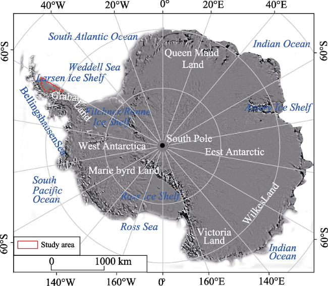
Figure 1 Location of the study area in the Antarctica. The underlying images are MODIS mosaics that are preprocessed by Haran et al. (2005).
The large pixels (250 m × 250 m) may smooth over small features that might be used for feature tracking such as those within grounding line areas or inlet glaciers where ice flows are confined in narrow valleys (Rott et al., 2011). For such cases, the texture in grounding line areas and inlet glaciers may not be observed and matched. Therefore, MODIS images may not be suitable to accurately retrieve velocity field within the grounding line areas. For successful feature tracking, the image pixel should be smaller than the surface displacements during the observation period, the time interval of image pair should be 2.2-3.7 years. The displacement between features over 250 m during the observation period on images corresponds to a surface velocity greater than 113 ma-1. Combining the two conditions mentioned above, we will only consider the floating ice areas with relatively high velocities or high quality of features in MODIS images, and mask out the grounding line areas where there is a lack of large-scale structural features for tracking. To define the study area, we will use the ice shelf fronts in 2000, 2003, 2006, 2009 and 2012, respectively, and the western edges to form the boundary of the study area (Figure 2). Once the boundary is defined, the total area of the study region is found to be approximately 46,000 km2.
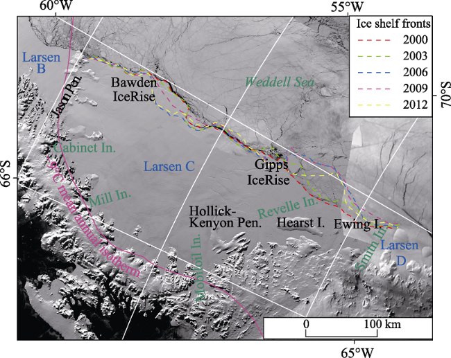
Figure 2 The ice shelf fronts in 2000, 2003, 2006, 2009 and 2012, respectively. The underlying images are MODIS mosaic in 2000.

3 Data sources

The input optical images to the COSI-Corr module in ENVI for glacier dynamics study need to meet two requirements: (1) at least two images at different times are needed so as to observe the significant flowing texture, and (2) the image pixel should be smaller than the surface displacements of ice shelf during the observation period. Once the requirements are met, the cross-correlation calculation based on repeat optical images can be carried out (Erten et al., 2012). The average velocities of ice shelves in the northern Antarctic Peninsula are significantly higher than that of tributary glaciers. Thus, MODIS images of 250-m resolution should meet the matching requirement of feature tracking within ice shelves. MODIS images in polar regions have the merits of frequent coverage (e.g. several times per day) and with a relatively long history, making it easy to select quality images for long-term velocity estimation on a large scale.
The MODIS data are provided by US National Aeronautics and Space Administration (NASA). Based on the satellite platforms (either Terra or Aqua), the data products are named differently: MOD02 for MODIS on Terra and MYD02 for MODIS on Aqua. MODIS L1B product consists of calibrated radiances at different resolutions (i.e., 1km, 500m, and 250m) and onboard calibrator/engineering data. These data are “scientific data”. The position information for each pixel is “geographic data”. We separated geographic data from the scientific data so that the scientific data images can be manipulated while keeping the geographic data intact. After processing, the scientific data are connected back to the geolocation data for geocoding. The final images (e.g. the pixel values are reflectance) have the geolocation accuracy of 50 m at nadir (Wolfe et al., 2002). It is higher than that of TM/ETM images, whose geolocation accuracy is 250 m (NASA, 1996). Here, we select band 1 images (e.g. spectral range: 620-670 nm; spatial resolution: 250 m) of MOD02 with minimum cloud and high quality of features in 2000, 2003, 2006, 2009 and 2012, respectively (Table 1). The displacements were extracted from the different image pairs with different time interval and the flowing velocity was then calculated. Finally, the velocity field over the Larsen C and southerly neighbours was generated by digital mosaicking.
Table 1 MODIS L1B images used for the velocity estimation and their parameters
Period1 Period2 Period3 Period4 Period5
27-MAR-2000 (13:15) 10-FEB-2003 (12:45) 3-JAN-2006 (12:30) 8-APR-2009 (14:15) 19-JAN-2012 (13:25)
29-MAR-2000 (13:05) 20-MAR-2003 (13:45) 5-JAN-2006 (14:45) 1-JAN-2009 (13:10) 25-JAN-2012 (12:50)
24-AUG-2000 (14:15) 8-APR-2003 (14:15) 7-JAN-2006 (14:20) 21-FEB-2012 (14:10)
26-AUG-2000 (15:40) 18-APR-2003 (14:50) 20-FEB-2006 (12:15) 19-AUG-2012 (13:50)
24-SEP-2000 (11:55) 11-DEC-2003 (14:50) 10-NOV-2006 (12:35) 23-AUG-2012 (13:25)
The ASTER Global Digital Elevation Model (GDEM) were generated based on paired stereo images in the near-infrared band obtained using the vertically downward and rear-view imaging sensors of ASTER onboard Terra (Cook et al., 2012). These data have a spatial resolution of 30 m and are horizontally georeferenced to Universal Transverse Mercator Projection/World Geodetic System 1984 (UTM/WGS84) with a coverage range of all land areas between 83°N and 83°S, corresponding to 99% of the land surface of the Earth (Hirt et al., 2010). We calculated the three-dimensional velocities based on the slope and aspect for the ice shelves extracted from the ASTER GDEM data.

4 Methods

4.1 Feature tracking

The COSI-Corr module in ENVI uses at least two MODIS images at different times for cross-correlation calculation. The early images (the reference images) are divided into matching windows (reference chip) by grids; each window of the same size (search chip) searches for the highest correlation in late images (the search images). The available cross-correlation algorithms include normalized cross-correlation (NCC) (Kaufmann and Ladstädter, 2003), orientation correlation (OC) (Fitch et al., 2002), cross-correlation operated in the Fourier domain (CCF) (McClellan et al., 2003), and the cross-correlation coefficient (CCC) (Evans, 2000). We identify the spatiotemporal patterns of surface movement of ice shelves for long-term velocity estimation on a large scale. Thus, the simplicity of CCC should meet the criteria of cross-correlation calculation. In this study we calculate the CCC as follows:
where f(x, y) and g(x, y) indicate the pixel value of feature points in the reference chip and search chip, respectively. u, v are surface offsets between reference chip of the reference image and search chip of the search image. 
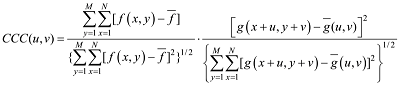
are mean pixel values of reference chip and search chip. N, M indicate the scopes of a chip. [f(x, y)- ] and [g(x+u, y+v)- (u, v)] indicate the pixel reflectance value that has the highest deviation between the means of all pixels which shall be identified as feature points from the chip. When difference in the overall reflectance of two images acquired at different times occurs, e.g., due to topography, orbits and altitude, the CCC automatically reduces the impact since only the deviation values rather than the absolute reflectance values are used. Nonetheless, this algorithm could cause mismatch since the criteria to identify a feature point is too restrictive. In the CCC algorithm, the calculated results are recorded using the S-N and W-E surface offsets, then we calculate the direction of ice shelf movement as follows:
where θ represents direction of ice flow within 0-360°; u is the W-E displacement, where from west to east is defined as positive; and v is the S-N displacement, where from south to north is defined as positive. Additionally, the signal-to-noise ratio (SNR) is used as a measure that expresses the reliability of a match to discriminate between correct and erroneous matches (Huang and Li, 2011), we set the threshold to be SNR < 0.8 and remove all results with SNR ≥ 0.8 to ensure quality in selecting matching pairs.
The parameter setting is an important step of COSI-Corr (Xu et al., 2011). The window size should be set small enough to prevent different ice displacements from being included in the same window, for areas with good contrast, and a window of 15 × 15 pixels can give correct matches based on MODIS images. However, the root mean square error (RMSE) of the displacement measurements over bare rocks is relatively high (Haug et al., 2010). Thus, to ensure the accuracy of calculations, the window size should be large enough and more pixels should be calculated. Different window sizes lead to calculated results with different SNR and RMSE. When the reference window (chip) is set to below 10 × 10 pixels, the noise from mismatches play a key role (Huang and Li, 2011), which shows random results; while when SNR increases gradually as window size grows, the velocities become stable. Meanwhile, the RMSE of the measurements increases with growth of size. Therefore, the reference window should be selected with a moderate size. Additionally, the window setting is according to the displacement of ice sheet or glacier, the highest velocity of ice shelves in the northern Antarctic Peninsula is approximately 700 ma-1. Thus, Haug et al. (2010) used matching windows of 44 × 44 pixels (11,000 m) for the MODIS images and 350 × 350 pixels (10,500 m) for the Landsat images in Larsen C ice shelf. Based on lots of experiments in the present study, the reference window (chip) size for cross-correlation calculation is set to 36 × 36 pixels, corresponding to a ground area of 9000 m × 9000 m, which can provide surface velocity with the best precision on the study area and the search area of the search image is set to 108 × 108 pixels, corresponding to a ground area of 27,000 m × 27,000 m.

4.2 Error analysis

The method of using CCC and MODIS images to derive ice velocity field on ice shelves can achieve satisfactory results; however, the velocity field derived is relatively coarse and noisy compared to other methods such as InSAR (Nakamura et al., 2007), feature tracking based on high-resolution optical image (Roland and Jason, 2013), and GPS (Testut et al., 2003). There are several sources of errors in the correlation calculations. For instance, the geolocation accuracy for MODIS imagery is 50 m (Wolfe et al., 2002), nonetheless, we find that the registration accuracy of image-to-image is better than 10 m from some primary experiments, and this results in an uncertainty of ±10 m. Another possible source of errors is related to feature point defects, e.g. matching of repeat MODIS images relies on surface contrast features (moraine deposits, ice mounds, etc.) that are usually scarce on the ice shelves. In addition, the accumulated snow pack can bury surface contrast features. Moreover, the vertical variations caused by oceanic tides and basal melt can cause erroneous matches near the eastern edges of the ice shelf (Yu et al., 2010).
The limitations discussed above can impact the accuracy of the surface velocity estimation for ice shelves. There are no stable bare rocks in the study area, thus testing objects outside the study area are selected for the error analysis. To quantify the uncertainties of the results in applying COSI-Corr to MODIS L1B images, 25 matching points are selected and investigated, the RMSE of the matching measurements in both W-E and S-N directions over stable bare rocks is given in Table 2. Results indicate that the average of the errors is approximately ±79 m which are slightly higher than the results reported by Haug et al. (2010) using the OC based on MODIS. This may be because the CCC has more erroneous matches. However, taking into account the fact that the study area has a vast expanse of approximately 46,000 km2, and a relatively high flow rate (in a range between 140 and 736 m/a), the uncertainties still meet the requirements for analysing the spatiotemporal variations of surface velocity. In short, the method of using CCC and MODIS images is suitable for the studies on the spatiotemporal variations of ice shelf movement on a large scale.
Table 2 Root mean square errors of displacement measurements obtained using the cross-correlation coefficient (CCC) over stable bare rocks
Image pairs RMSEE-W (m) RMSES-N (m)
2000/2003 54 62
2003/2006 46 56
2006/2009 61 71
2009/2012 47 52
Mean 52 60

5 Results

5.1 Spatial pattern of surface velocities

The surface velocity fields of ice shelves in the northern Antarctic Peninsula over four periods are obtained by the cross-correlation of four sets of images. The results show that the ice flow directions generally match the peninsula’s pattern and the crevasse distribution. Ice mainly flows eastward into the Weddell Sea (Figure 3).
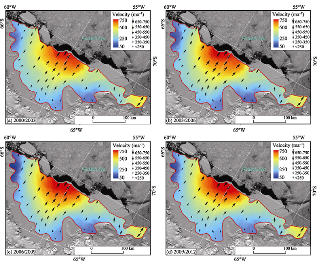
Figure 3 Spatial pattern of surface velocity of ice shelves in the northern Antarctic Peninsula during four periods (a. 2000/2003, b. 2003/2006, c. 2006/2009, and d. 2009/2012). The arrows in black indicate flow vector with quantities and directions at the 50 sample points with the best contrast on MODIS images (Figure 4). The underlying images are MODIS mosaic in 2006.
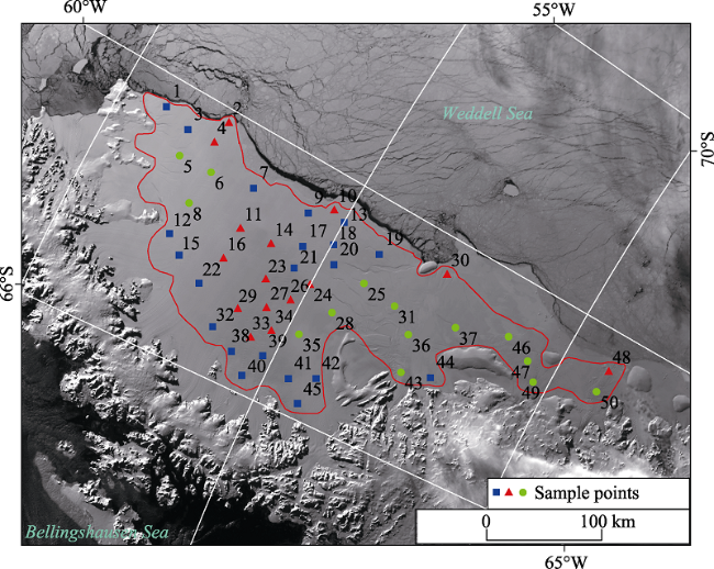
Figure 4 Sketch map of 50 sample points. The ice at the sample points in blue shows a continuous acceleration; at the sample points in red shows that there is not any significant change in velocity; and at the sample points in green shows a deceleration from the period 2006-2009 to the period 2009-2012. The underlying images are MODIS mosaic in 2009.
As observed, the spatial pattern of the velocity field exhibits an increasing trend from the western grounding line to the maximum at the middle part of the ice shelf front on Larsen C, and the velocity field shows relatively higher values in its southerly neighboring ice shelf
(e.g. Smith Inlet). As expected, we find the highest velocities at the central to outer part of the Larsen C ice shelf, with velocities exceeding 700 ma-1. The absolute velocity value at those locations varies greatly from 141 ma-1 at one location to up to 736 ma-1 at another location, indicating the heterogeneity of the spatial distribution of the speed field of the ice shelves. Within the area of collectively homogeneous flow pattern, some irregularities can still be identified that correspond to fractures spatially, together with a remarkable imprint indicated on the ice motion field where rifts lie on the Hollick-Kenyon Pen. and the Hearst I. (Figure 2). In addition, a few high velocity-gradient zones are also present, for example, from the Mill Inlet and Cabinet Inlet to Bawden Ice Rise. From the Mobiloil Inlet and Smith Inlet to outer part of ice shelf, the velocities between 100 and 150 ma-1 are higher than those of the neighboring regions.

5.2 Temporal variations in surface velocities

Fifty sample points with the best contrast almost evenly distributed across the study area (Figure 3) are selected for quantitative analysis and they are marked in Figure 4. Figure 5 shows the velocity values derived from various periods at each location. We can see that at most locations, the ice speed increased from 2000-2003 to 2009-2012 (Figure 5).
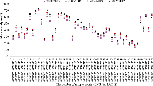
Figure 5 The mean velocity of 50 sample points with latitude and longitude during four periods
More specifically, the mean velocity of 50 sample points in 2000-2003 is 397 ma-1 with the range between 141 and 711 ma-1. Meanwhile, the mean velocity in 2003-2006 is 424 ma-1, and the range is between 158 to 709 ma-1. The mean velocity in 2006-2009 is 444 ma-1 with the range between 175 to 706 ma-1. The mean velocity in 2009-2012 is 445 ma-1 and the range is between 183 to 736 ma-1 (Figure 5). Results show that the ice flows relatively slowly in the inner regions of the ice shelf, e.g., the five sample points (31, 36, 37, 43 and 44) in the Hollick-Kenyon Pen. and Hearst I. (e.g. mean velocity is 236-285 ma-1). The three sample points (1, 3 and 5) in the northern Larsen C Ice Shelf show even lower velocity. In contrast, the sample points (9, 10, 13 and 18) in the middle section of the ice front on Larsen C Ice Shelf have higher velocities of 653-704 ma-1, and the sample points (48 and 50) in the Smith Inlet also have high velocities of 608-649 ma-1.
Overall, temporal changes in surface velocities at the 50 sample points show continuous acceleration from 2000 to 2012. They increased by up to 12% from 2000-2003 to 2009-2012. The overall velocity on ice shelf inlet and outer part of Larsen C shows a continuous increase. The Mobiloil inlet, Mill inlet, etc. did not appear to respond to the acceleration and deceleration of the eastern ice shelf edge, and ice at points 22 and 40, etc. in this region shows a continuous and steady rate of acceleration. The trend of the velocities on the eastern ice shelf edge (at sample points 10, 30 and 48) is inconclusive, due to effects of oceanic tides and basal melt. The temporal variations show a widespread deceleration on the southern Larsen C Ice Shelf from 2006-2009 to 2009-2012, as well as its neighboring ice shelves (e.g. the Smith Inlet). The ice deceleration observed in these regions is consistent with the study by Khazendar et al. (2011). Ice at 10 points in the southern Larsen C and its neighboring ice shelves has been decelerating from 2006-2009 to 2009-2012 by up to 2.5%. Overall, temporal changes in surface velocities show a continuous acceleration from 2000 to 2012 (Figure 6), whereas the acceleration rate during 2000-2009 is relatively higher than that during 2009-2012.
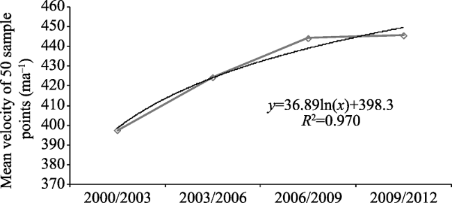
Figure 6 Variation of mean velocity of 50 sample points during 2000-2012

6 Discussion

The matching method is one of the important factors that impact the uncertainty of the surface velocity derived from MODIS images. Heid and Kääb (2012) compared and evaluated different existing matching methods and showed that for areas with high visual contrast on optical images, NCC performs better than other methods with slightly lower RMSE. However, Haug et al. (2010) reported that NCC produces more incorrect matches than OC but with similar RMSE, and the uncertainty of NCC and OC is ±21.5 m and ±21.8 m, respectively. CCC is often used to derive glacier velocity field due to the algorithm’s simplicity (Huang and Li, 2011). The main rule of CCC is similar to NCC, thus this matching method is also suitable for deriving velocity in areas with good visual contrast on images (e.g. on open areas of ice shelf where there are significant flowing textures and large-scale structural features). In addition, for areas with relatively high velocity, using CCC and MODIS images can get acceptable errors, with the RMSE being approximately ±79 m which is just slightly higher than the results reported by Haug et al. (2010) by using the OC. We identify the spatiotemporal patterns of surface movement of ice shelves for long-term velocity estimation on a large scale. Thus, the CCC meets the requirements for analysing the spatiotemporal variations on ice shelves in the northern Antarctic Peninsula, which can serve as a supplement to the existing methods.
In line with existing studies, and comparing with the Larsen B ice shelf, our study shows a continuous but moderate increase in speed on large portions of the study area. The overall velocity over the whole study area increased approximately by 12% from 2000 to 2012, while the rate of acceleration in the northern sector is higher as compared to the southern sector. The estimated differences in speed between 2000 and 2012 can be divided into three groups (Figure 4): 1) Northern sector: This region shows a continuous acceleration during the observation period, possibly due to a reduction in backstress from the Bawden Ice Rise and/or the erosion of marine ice formerly suturing parallel flow bands together (McGrath et al., 2012). While the essential reason for the drastic acceleration is related to the condition that this region has progressively thinned, the elevation of the Larsen C has lowered at a rate of 0.06-0.09 ma-1 during 1978-2008 (McGrath et al., 2012), and the greatest lowering occurred in the northern sector of Larsen C (Fricker and Padman, 2012; Shepherd et al., 2003). This lowering circumstance is dominated by the increased melt-water production/refreezing (Holland et al., 2011) rather than increased basal melting. 2) Southern sector: Many large surface crevasses originate at Kenyon Peninsula and end at Gipps Ice Rise, this region and neighboring ice shelf extending to the south show an overall acceleration during the observation period. Beyond our expectation, the present estimated results show that the southern sector slowed down slightly during recent years. This deceleration should be related to the increase of backstress caused by the ice fronts which tend to be more stabilized recently. Additionally, the southern sector is a more complex region, with the overall surface elevation showing a slight increase during the period 1993-2005. (Fricker and Padman, 2012). 3) The floating ice region near the grounding line: We mask out the grounding line area due to the coarse spatial resolution of MODIS images. This region mainly covers Cabinet Inlet, Mill Inlet, Mobiloil Inlet, Revelle Inlet and Smith Inlet, etc. The northern sector of the Larsen C accelerated by 15% between 2000 and 2006, and a further acceleration of 6%-8% between 2006 and 2008 at the nearby grounding line areas (e.g. Cabinet Inlet) (Khazendar et al., 2011). Smith Inlet shows a deceleration during recent years. The temporal characteristics of surface velocity in the floating ice region near the grounding line show a continuous and steady rate of acceleration, where did not appear to respond to the acceleration and deceleration of the eastern ice shelf edge. This acceleration is possibly caused by reduction of backstress and increasing of longitudinal stress with downstream ice shelves progressively thinned (Scambos et al., 2003). Despite the ice shelves in the northern Antarctic Peninsula will not face imminent collapse (Holland et al., 2015), they are undergoing significant acceleration in speed which is spatially related to fracture and thinning (Khazendar et al., 2011). The continuous acceleration in speed and thinning in elevation, increasing basal melt due to warming upper-ocean temperatures (Nicholls et al., 2004), and the meltwater-driven crevasse propagation are the main mechanism for the rapid collapse of ice shelf (Rott et al., 1996; Scambos et al., 2000, 2009). It presages destabilization if Larsen C is to evolve similarly to Larsen B (Griggs and Bamber, 2009).

7 Conclusions

This study estimates the surface velocities in ice shelves of the northern Antarctic Peninsula using COSI-Corr module and MODIS images in 2000, 2003, 2006, 2009 and 2012, respectively. The results show that the overall velocity of ice shelves is relatively high due to the extremely large ice flux, and it has a mean velocity of approximately 400 ma-1 with a maximum of 736 ma-1, making it one of the fastest-moving areas in the Antarctic Peninsula. The spatial pattern of the velocity field shows that velocities increase from the western grounding line to a maximum of approximately 700 ma-1 at the middle region of the ice front on Larsen C Ice Shelf and the ice flows relatively slowly in the inner parts. Temporal changes of surface velocities show a continuous acceleration from 2000 to 2012, and the acceleration rate from 2000-2003 to 2006-2009 is greater than that from 2006-2009 to 2009-2012. However, the velocity on the southern Larsen C Ice Shelf and the Smith Inlet from 2009 to 2012 shows a deceleration. The method of using CCC and MODIS images to derive ice velocity field for ice shelves only provides moderate accuracy due to the simplicity of cross-correlation algorithm, feature point defects and geolocation errors, etc. However, these uncertainties still meet the requirements for analysing the spatiotemporal variations of surface velocity. In short, the method of using CCC and MODIS images is suitable for large-scale monitoring of ice velocities in the Antarctic ice shelves, which is a valuable complement to other methods such as INSAR, GPS and high-resolution optical image feature tracking, etc.

The authors have declared that no competing interests exist.

1
Ahn Y, Howat I M, 2010. Efficient automated glacier surface velocity measurement from repeat images using multi-image/multichip and null exclusion feature tracking.IEEE Transactions on Geoscience and Remote Sensing, 49(8): 2838-2846.

2
Ayoub F, Leprince S, Avouac J P, 2009. Co-registration and correlation of aerial photographs for ground deformation measurements.ISPRS Journal of Photogrammetry and Remote Sensing, 64(6): 551-560.<h2 class="secHeading" id="section_abstract">Abstract</h2><p id="">We describe and test a procedure to accurately co-register and correlate multi-temporal aerial images. We show that this procedure can be used to measure surface deformation, and explore the performance and limitations of the technique. The algorithms were implemented in a software package, COSI-Corr (available from the Caltech Tectonics Observatory website). The technique is validated on several case examples of co-seismic deformation. First, we measure co-seismic ground deformation due to the 1992, Mw 7.3, Landers, California, earthquake from 1 m resolution aerial photography of the National Aerial Photography Program (United States Geological Survey). The fault ruptures are clearly detected, including small kilometric segments with fault slip as small as a few tens of centimeters. We also obtained similar performance from images of the fault ruptures produced by the 1999 Mw 7.1 Hector Mine, California, earthquake. The measurements are shown to be biased due to the inaccuracy of the Digital Elevation Model, film distortions, scanning artifacts, and ignorance of ground displacements at the location of the tie points used to co-register the multi-temporal images. We show that some of these artifacts can be identified and corrected.</p>

DOI

3
Berthier E, Raup B, Scambos T, 2003. New velocity map and mass-balance estimate of Mertz Glacier, East Antarctica, derived from Landsat sequential imagery.Journal of Glaciology, 49(167): 503-511.Automatic feature tracking on two Landsat images (acquired in January 2000 and December 2001) generates a complete and accurate velocity field of Mertz Glacier, East Antarctica. This velocity field shows two main tributaries to the ice stream. Between the tributaries, a likely obstruction feature in the bedrock results in a slow-down of the flow. A third Landsat image, acquired in 1989 and combined with the 2000 image, permits the determination of the glacier mean velocity during the 1990s. Although some parts of the Mertz Glacier system show evidence of slight speed increase, we conclude that the Mertz flow speed is constant within our uncertainty (35 m a). Using this complete velocity field, new estimates of the ice discharge flux, 17.8 kma(16.4 Gt a), and of the basal melting of the tongue, 11m aof ice, are given. Our results lead to an apparent imbalance of the drainage basin (ice discharge 3.5 kmalower than the accumulation). Considering previous studies in the Mertz Glacier area, we then discuss the uncertainty of this imbalance and the problems with accumulation mapping for this region

DOI

4
Bindschadler R A, Fahnestock M A, Skvarca Pet al., 1994. Surface-velocity field of the northern Larsen Ice Shelf, Antarctica.Annals of Glaciology, 20(1): 319-326.

5
Broeke M V D, 2005. Strong surface melting preceded collapse of Antarctic Peninsula ice.Geophysical Research Letters, 32(12): L12185.

6
Cook A J, Vaughan D G, 2010. Overview of areal changes of the ice shelves on the Antarctic Peninsula over the past 50 years. The Cryosphere, 4(1): 77-98.The article provides information on the areal changes of the ice shelves in the Antarctic Peninsula (AP) over the past 50 years before 2010. It presents an overview of the characteristics of the twelve ice shelves on the AP during the covered period as well as the overall reduction in total ice-shelf by over 28,000 kilometer. It explores the features of each ice shelf, and examines its spacial and temporal patterns in accordance to the timing and rate of retreat.

DOI

7
Cook A J, Murray T, Luckman Aet al., 2012. A new 100-m Digital Elevation Model of the Antarctic Peninsula derived from ASTER Global DEM: Methods and accuracy assessment.Earth System Science Data, 4(1): 129-142.A high resolution surface topography Digital Elevation Model (DEM) is required to underpin studies of the complex glacier system on the Antarctic Peninsula. A complete DEM with better than 200 m pixel size and high positional and vertical accuracy would enable mapping of all significant glacial basins and provide a dataset for glacier morphology analyses. No currently available DEM meets these specifications. We present a new 100-m DEM of the Antarctic Peninsula (63-70 S), based on ASTER Global Digital Elevation Model (GDEM) data. The raw GDEM products are of high-quality on the rugged terrain and coastal-regions of the Antarctic Peninsula and have good geospatial accuracy, but they also contain large errors on ice-covered terrain and we seek to minimise these artefacts. Conventional data correction techniques do not work so we have developed a method that significantly improves the dataset, smoothing the erroneous regions and hence creating a DEM with a pixel size of 100 m that will be suitable for many glaciological applications. We evaluate the new DEM using ICESat-derived elevations, and perform horizontal and vertical accuracy assessments based on GPS positions, SPOT-5 DEMs and the Landsat Image Mosaic of Antarctica (LIMA) imagery. The new DEM has a mean elevation difference of -4 m ( 25 m RMSE) from ICESat (compared to -13 m mean and 97 m RMSE for the original ASTER GDEM), and a horizontal error of less than 2 pixels, although elevation accuracies are lower on mountain peaks and steep-sided slopes. The correction method significantly reduces errors on low relief slopes and therefore the DEM can be regarded as suitable for topographical studies such as measuring the geometry and ice flow properties of glaciers on the Antarctic Peninsula. The DEM is available for download from the NSIDC website: http://nsidc.org/data/nsidc-0516.html (doi:10.5060/D47P8W9D).

DOI

8
Erten E, Chesnokova O, Hajnsek Iet al., 2012. Glacier surface velocity measure based on polarimetric tracking. Geoscience and Remote Sensing Symposium (IGARSS),2012 IEEE International, 12: 3126-3129.

9
Evans A N, 2000. Glacier surface motion computation from digital image sequences.IEEE Transactions on Geoscience and Remote Sensing, 38(2): 1064-1072.Not Available

DOI

10
Fitch A J, Kadyrov A, Christmas W J et al., 2002. Orientation Correlation, in: British Machine Vision Conference, 133-142.

11
Fricker H A, Padman L, 2012. Thirty years of elevation change on Antarctic Peninsula ice shelves from multimission satellite radar altimetry.Journal of Geophysical Research,117: C02026.Abstract Top of page Abstract 1.Introduction 2.Data 3.Methods 4.Results 5.Discussion 6.Conclusions AppendixA::Intramission Crossover Analysis Acknowledgments References Supporting Information [1] We use data acquired between 1978 and 2008 by four satellite radar altimeter missions (Seasat, ERS-1, ERS-2 and Envisat) to determine multidecadal elevation change rates ( dh i / dt ) for six major Antarctic Peninsula (AP) ice shelves. In areas covered by the Seasat orbit (to 72.16°S), regional-averaged 30-year trends were negative (surface lowering), with rates between 610.03 and 610.16 m a 611 . Surface lowering preceded the start of near-continuous radar altimeter operations that began with ERS-1 in 1992. The average rate of lowering for the first 14 years of the period was typically smaller than the 30-year average; the exception was the southern Wilkins Ice Shelf, which experienced negligible lowering between 2000 and 2008, when a series of large calving events began. Analyses of the continuous ERS/Envisat time series (to 81.5°) for 1992–2008 reveal a period of strong negative dh i / dt on most ice shelves between 1992 and 1995. Based on prior studies of regional atmospheric and oceanic conditions, we hypothesize that the observed elevation changes on Larsen C Ice Shelf are driven primarily by firn compaction while the western AP ice shelves are responding to changes in both surface mass balance and basal melt rates. Our time series also show that large changes in dh i / dt can occur on interannual time scales, reinforcing the importance of long time series altimetry to separate long-term trends associated with climate change from interannual to interdecadal natural variability.

DOI

12
Glasser N F, Kulessa B, Luckman Aet al., 2009. Surface structure and stability of the Larsen C ice shelf, Antarctic Peninsula.Journal of Glaciology, 55(191): 400-410.A structural glaciological description and analysis of surface morphological features of the Larsen C ice shelf, Antarctic Peninsula, is derived from satellite images spanning the period 1963-2007. The data are evaluated in two time ranges: a comparison of a 1963 satellite image photomosaic with a modern digital mosaic compiled using 2003/04 austral summer data; and an image series since 2003 showing recent evolution of the shelf. We map the ice-shelf edge, rift swarms, crevasses and crevasse traces, and linear longitudinal structures (called 'flow stripes' or 'streak lines'). The latter are observed to be continuous over distances of up to 200 km from the grounding line to the ice-shelf edge, with little evidence of changes in pattern over that distance. Integrated velocity measurements along a flowline indicate that the shelf has been stable for ~560 years in the mid-shelf area. Linear longitudinal features may be grouped into 12 units, each related to one or a small group of outlet feeder glaciers to the shelf. We observe that the boundaries between these flow units often mark rift terminations. The boundary zones originate upstream at capes, islands or other suture areas between outlet glaciers. In agreement with previous work, our findings imply that rift terminations within such suture zones indicate that they contain anomalously soft ice. We thus suggest that suture zones within the Larsen C ice shelf, and perhaps within ice shelves more generally, may act to stabilize them by reducing regional stress intensities and thus rates of rift lengthening.

DOI

13
Griggs J A, Bamber J L, 2009. Ice shelf thickness over Larsen C, Antarctica, derived from satellite altimetry.Geophysical Research Letters, 36(19): L19501.Satellite radar altimetry can be used to infer the thickness of floating ice shelves around Antarctica under the assumption of hydrostatic equilibrium. Ice shelf thickness is an essential parameter in mass budget calculations and is one of the more poorly characterised. Using data from the ERS-1 radar altimeter recorded in 1994-5, we calculate the thickness of Larsen C ice shelf on the Antarctic Peninsula. The surface elevation was determined to an accuracy of -2.3 卤 4.35 m as compared to elevations from the laser altimeter onboard ICESat. Using a model for firn depth and density, we created a 1 km grid of ice shelf thickness for Larsen C. The accuracy of the ice thickness retrieval was determined from independent airborne radio echo sounding data. The results indicated a bias of -0.22 m and random error of 36.7 m, which is equivalent to 12.7% of the mean thickness for this ice shelf.

DOI

14
Haran T, Bohlander J, Scambos T Aet al., 2005. MODIS mosaic of Antarctica (MOA) image map, digital media, Natl. National Snow and Ice Data Center (US), Boulder, Colo.

15
Haug T, Kääb A, Skvarca P, 2010. Monitoring ice shelf velocities from repeat MODIS and Landsat data-a method study on the Larsen C ice shelf, Antarctic Peninsula, and 10 other ice shelves around Antarctica.The Cryosphere, 4(2): 161-178.

16
Heid T, Kääb A, 2012. Evaluation of existing image matching methods for deriving glacier surface displacements globally from optical satellite imagery.Remote Sensing of Environment, 118: 339-355.Automatic matching of images from two different times is a method that is often used to derive glacier surface velocity. Nearly global repeat coverage of the Earth's surface by optical satellite sensors now opens the possibility for global-scale mapping and monitoring of glacier flow with a number of applications in, for example, glacier physics, glacier-related climate change and impact assessment, and glacier hazard management. The purpose of this study is to compare and evaluate different existing image matching methods for glacier flow determination over large scales. The study compares six different matching methods: normalized cross-correlation (NCC), the phase correlation algorithm used in the COSI-Corr software, and four other Fourier methods with different normalizations. We compare the methods over five regions of the world with different representative glacier characteristics: Karakoram, the European Alps, Alaska, Pine Island (Antarctica) and southwest Greenland. Landsat images are chosen for matching because they expand back to 1972, they cover large areas, and at the same time their spatial resolution is as good as 15 m for images after 1999 (ETM+pan). Cross-correlation on orientation images (CCF-O) outperforms the three similar Fourier methods, both in areas with high and low visual contrast. NCC experiences problems in areas with low visual contrast, areas with thin clouds or changing snow conditions between the images. CCF-O has problems on narrow outlet glaciers where small window sizes (about 16 pixels by 16 pixels or smaller) are needed, and it also obtains fewer correct matches than COSI-Corr in areas with low visual contrast. COSI-Corr has problems on narrow outlet glaciers and it obtains fewer correct matches compared to CCF-O when thin clouds cover the surface, or if one of the images contains snow dunes. In total, we consider CCF-O and COSI-Corr to be the two most robust matching methods for global-scale mapping and monitoring of glacier velocities. If combining CCF-O with locally adaptive template sizes and by filtering the matching results automatically by comparing the displacement matrix to its low pass filtered version, the matching process can be automated to a large degree. This allows the derivation of glacier velocities with minimal (but not without!) user interaction and hence also opens up the possibility of global-scale mapping and monitoring of glacier flow.

DOI

17
Hirt C, Filmer M, Featherstone W, 2010. Comparison and validation of the recent freely available ASTER-GDEM ver1, SRTM ver4.1 and GEODATA DEM-9S ver3 digital elevation models over Australia.Australian Journal of Earth Sciences, 57(3): 337-347.

18
Holland P R, Brisbourne A, Corr H F Jet al., 2015. Oceanic and atmospheric forcing of Larsen C Ice-Shelf thinning.The Cryosphere, 9(3): 1005-1024.The catastrophic collapses of Larsen A and B ice shelves on the eastern Antarctic Peninsula have caused their tributary glaciers to accelerate, contributing to sea-level rise and freshening the Antarctic Bottom Water formed nearby. The surface of Larsen C Ice Shelf (LCIS), the largest ice shelf on the peninsula, is lowering. This could be caused by unbalanced ocean melting (ice loss) or enhanced firn melting and compaction (englacial air loss). Using a novel method to analyse eight radar surveys, this study derives separate estimates of ice and air thickness changes during a 15-year period. The uncertainties are considerable, but the primary estimate is that the surveyed lowering (0.066 ± 0.017 m yr611) is caused by both ice loss (0.28 ± 0.18 m yr611) and firn-air loss (0.037 ± 0.026 m yr611). The ice loss is much larger than the air loss, but both contribute approximately equally to the lowering because the ice is floating. The ice loss could be explained by high basal melting and/or ice divergence, and the air loss by low surface accumulation or high surface melting and/or compaction. The primary estimate therefore requires that at least two forcings caused the surveyed lowering. Mechanisms are discussed by which LCIS stability could be compromised in the future. The most rapid pathways to collapse are offered by the ungrounding of LCIS from Bawden Ice Rise or ice-front retreat past a "compressive arch" in strain rates. Recent evidence suggests that either mechanism could pose an imminent risk.

DOI

19
Holland P R, Corr H F J, Pritchard H Det al., 2011. The air content of Larsen Ice Shelf.Geophysical Research Letters, 38(10): L10503.The air content of glacial firn determines the effect and attribution of observed changes in ice surface elevation, but is currently measurable only using labor-intensive ground-based techniques. Here a novel method is presented for using radar sounding measurements to decompose the total thickness of floating ice shelves into thicknesses of solid ice and firn air (or firn water). The method is applied to a 1997/98 airborne survey of Larsen Ice Shelf, revealing large spatial gradients in air content that are consistent with existing measurements and local meteorology. The gradients appear to be governed by meltwater-induced firn densification. We find sufficient air in Larsen C Ice Shelf for increased densification to account for its previously observed surface lowering, and the rate of lowering superficially agrees with published trends in melting. This does not preclude a contribution to the lowering from oceanic basal melting, but a modern repeat of the survey could conclusively distinguish atmosphere-led from ocean-led change. The technique also holds promise for the calibration of firn-density models, derivation of ice thickness from surface elevation measurements, and calculation of the sea-level contribution of changes in grounded-ice discharge.

DOI

20
Huang L, Li Z, 2011. Comparison of SAR and optical data in deriving glacier velocity with feature tracking.International Journal of Remote Sensing, 32(10): 2681-2698.Feature tracking is an efficient way to derive glacier velocity. It is based on a cross-correlation algorithm that seeks offsets of the maximal correlation windows on repeated satellite images. In this paper we demonstrate that different window sizes lead to different velocities. The averaged velocity gradient (AVG) method is proposed to improve window sizes in feature tracking and to obtain the most suitable flow field. The AVG method measures velocity variation between adjacent windows on the whole glacier in the image. Different window sizes lead to different AVG values, and the best-size window corresponds to the value where the AVG changes from abrupt to gradual. Using improved feature tracking, two flow fields of the same glacier are acquired with Advanced Land Observing Satellite (ALOS) optical and synthetic aperture radar (SAR) data, respectively. The advantages, application conditions, accuracy and disadvantages of the two kinds of data using the feature tracking method are discussed.

DOI

21
Jansen D, Kulessa B, Sammonds P Ret al., 2010. Present stability of the Larsen C ice shelf, Antarctic Peninsula.Journal of Glaciology, 56(198): 593-600.We modelled the flow of the Larsen C and northernmost Larsen D ice shelves, Antarctic Peninsula, using a model of continuum mechanics of ice flow, and applied a fracture criterion to the simulated velocities to investigate the ice shelf's present-day stability. Constraints come from satellite data and geophysical measurements from the 2008/09 austral summer. Ice-shelf thickness was derived from BEDMAP and ICESat data, and the density epth relationship was inferred from our in situ seismic reflection data. We obtained excellent agreements between modelled and measured ice-flow velocities, and inferred and observed distributions of rifts and crevasses. Residual discrepancies between regions of predicted fracture and observed crevasses are concentrated in zones where we assume a significant amount of marine ice and therefore altered mechanical properties in the ice column. This emphasizes the importance of these zones and shows that more data are needed to understand their influence on ice-shelf stability. Modelled flow velocities and the corresponding stress distribution indicate that the Larsen C ice shelf is stable at the moment. However, weakening of the elongated marine ice zones could lead to acceleration of the ice shelf due to decoupling from the slower parts in the northern inlets and south of Kenyon Peninsula, leading to a velocity distribution similar to that in the Larsen B ice shelf prior to its disintegration.

DOI

22
Kaufmann V, Ladstädter R, 2003. Quantitative analysis of rock glacier creep by means of digital photogrammetry using multitemporal aerial photographs: Two case studies in the Austrian Alps.Proceedings of the 8th International Conference on Permafrost, 525-530.

23
Kääb A, Vollmer M, 2000. Surface geometry, thickness changes and flow fields on creeping mountain permafrost: Automatic extraction by digital image analysis.Permafrost and Periglacial Processes, 11(4): 315-326.

24
Ke C Q, Kou C, Ludwig Ret al., 2013. Glacier velocity measurements in the eastern Yigong Zangbo basin, Tibet, China. Journal of Glaciology, 59(218): 1060-1068.We apply the feature-tracking method to L-band synthetic aperture radar (SAR) images to derive detailed motion patterns of glaciers in the Yigong Zangbo basin during summer 2007. The results indicate that the flow patterns are generally constrained by the valley geometry and terrain complexity. The mean velocities of the 12 glaciers were 15鈥206 m a, with a maximum of 423 m afor Glacier No. 5a. The majority of the glaciers exhibited high and low velocities in their upper and lower sections, respectively. The glacier area ranges from 3 to 42 km. It is found that velocity shows a positive correlation with the glacier area and length. Many small-scale temporal/spatial variations in the glacier flow patterns were observed along the central glacier flowline.

DOI

25
Khazendar A, Rignot E, Larour E, 2011. Acceleration and spatial rheology of Larsen C Ice Shelf, Antarctic Peninsula.Geophysical Research Letters, 38(9): L09502.The disintegration of several Antarctic Peninsula ice shelves has focused attention on the state of the Larsen C Ice Shelf. Here, we use satellite observations to map ice shelf speed from the years 2000, 2006 and 2008 and apply inverse modeling to examine the spatial pattern of ice-shelf stiffness. Results show that the northern half of the ice shelf has been accelerating since 2000, speeding up by 15% between 2000 and 2006 alone. The distribution of ice stiffness exhibits large spatial variations that we link to tributary glacier flow and fractures. Our results reveal that ice down-flow from promontories is consistently softer, with the exception of Churchill Peninsula where we infer a stabilizing role for marine ice. We conclude that although Larsen C is not facing imminent collapse, it is undergoing significant change in the form of flow acceleration that is spatially related to thinning and fracture.

DOI

26
Leprince S, Barbot S, Ayoub Fet al., 2007. Automatic and precise ortho-rectification, coregistration,and subpixel correlation of satellite images, application to ground deformation measurements.IEEE International Symposium on Geoscience and Remote Sensing, 45(6): 1529-1558.

27
Manson R, Coleman R, Morgan Pet al., 2000. Ice velocities of the Lambert Glacier from static GPS observations. Earth,Planets and Space, 52(11):1031-1036.

28
McClellan J, Schafer R, Yoder M, 2003. Signal Processing First.Pearson Prentice Hall: Pearson Education, Inc.0-13-120265-0.

29
McGrath D, Steffen K, Rajaram Het al., 2012. Basal crevasses on the Larsen C Ice Shelf, Antarctica: Implications for meltwater ponding and hydrofracture.Geophysical Research Letters, 39(16): L16504.A key mechanism for the rapid collapse of both the Larsen A and B Ice Shelves was meltwater-driven crevasse propagation. Basal crevasses, large-scale structural features within ice shelves, may have contributed to this mechanism in three important ways: i) the shelf surface deforms due to modified buoyancy and gravitational forces above the basal crevasse, creating >10 m deep compressional surface depressions where meltwater can collect, ii) bending stresses from the modified shape drive surface crevassing, with crevasses reaching 40 m in width, on the flanks of the basal-crevasse-induced trough and iii) the ice thickness is substantially reduced, thereby minimizing the propagation distance before a full-thickness rift is created. We examine a basal crevasse (4.5 km in length, 230 m in height), and the corresponding surface features, in the Cabinet Inlet sector of the Larsen C Ice Shelf using a combination of high-resolution (0.5 m) satellite imagery, kinematic GPS and in situ ground penetrating radar. We discuss how basal crevasses may have contributed to the breakup of the Larsen B Ice Shelf by directly controlling the location of meltwater ponding and highlight the presence of similar features on the Amery and Getz Ice Shelves with high-resolution imagery.

DOI

30
Morris E M, Vaughan D G, 2003. Spatial and temporal variation of surface temperature on the Antarctic Peninsula and the limit of viability of ice shelves, in Antarctic Peninsula Climate Variability, Historical and Paleoenvironmental Perspectives. In: Domack E et al. (eds.). Antarct. Res. Ser., 79: 61-68, AGU, Washington, D. C.Mapping surface air temperature in the Antarctic Peninsula region is made unusually difficult by: the scarcity of meteorological stations, strong climatic gradients and recent rapid regional warming. We have compiled a database of 534 mean annual temperatures derived from measurements of snow temperature at around 10-m depth and air temperature measured at meteorological stations and automatic weather stations. These annual temperatures were corrected for interannual variability using a composite record from six stations across the region. The corrected temperatures were then analysed using multiple linear regression to yield altitudinal and temporal lapse rates. A subset of 508 values were then used to produce a map of temperature reduced to sea level and for a specific epoch (2000 A.D.). The map shows the dramatic climate contrast (3-5degreesC) between the east and west coast of the Antarctic Peninsula in greater detail than earlier studies and also indicates that the present limit of ice shelves closely follows the -9degreesC (2000 A.D.) isotherm. Furthermore, the limit of ice shelves known to have retreated during the last 100 years is bounded by the -9degreesC and -5degreesC (2000 A.D.) isotherms, suggesting that the retreat of ice shelves in the Antarctic Peninsula region is consistent with a warming of around similar to 4 degrees C.

DOI

31
Nakamura K, Doi K, Shibuya K, 2007. Estimation of seasonal changes in the flow of Shirase Glacier using JERS-1/SAR image correlation.Polar Science, 1(2): 73-83.This paper presents estimates of detailed seasonal variations in ice-flow velocity for Shirase Glacier calculated using data obtained by Japanese Earth Resources Satellite-1 (JERS-1) synthetic aperture radar (SAR). We used 12 pairs of images (44-day repeat cycle) over the interval from 30 April 1996 to 1 July 1998 to estimate ice-flow fields using an image correlation method. Geometric registration was performed with reference to the RADARSAT Antarctic Mapping Project (RAMP) image dataset. Error analysis based on feature mismatch indicated an absolute error of ±0.3002km/a and relative error of ±0.0402km/a in the estimated flow velocity. The obtained ice-flow velocity increases rapidly from the upstream region (1.1802km/a) to the grounding line, where it becomes stagnant (2.3202km/a), before accelerating gradually to 2.62–2.8202km/a in the downstream region and then increasing to 3.05–3.5002km/a at the terminus of the floating ice tongue. The ice-flow velocities in the downstream region are highly variable, depending on both the distance from the grounding line and the observed epoch (season). Most of the obtained seasonal variations in ice-flow velocity at the floating ice tongue are within the range of the associated error estimate, but the annual difference between 1997 (3.1102km/a) and 1998 (3.5002km/a) is significant, reflecting a possible acceleration in the ice-flow velocity in association with the disappearance of the floating ice tongue between April and May of 1998. In terms of the summer–winter difference in averaged air temperature, the large difference recorded in 1997 (17.002°C) relative to 1996 (13.902°C) corresponds to a reduced ice-flow velocity in 1997 (approximately 0.2002km/a) relative to that in 1996 (approximately 0.3002km/a), indicating interactions between air, sea ice, and glacier flow in Lützow-Holm Bay.

DOI

32
NASAG, 1996. Landsat 7 System Specification, NASA Goddard Space Flight Center.

33
Nicholls K W, Pudsey C J, Morris P, 2004. Summertime water masses off the northern Larsen C Ice Shelf, Antarctica.Geophysical Research Letters, 31(9): L09309.We report on oceanographic observations made at the northern end of Larsen C Ice Shelf in the western Weddell Sea. It appears that the Larsen C continental shelf is flushed not by High Salinity Shelf Water from the southern continental shelf, but by Modified Weddell Deep Water (MWDW) flowing across the shelf break. MWDW is observed at the ice front, having tracked west along the northward facing slopes of depressions that reach to the shelf break. Ice Shelf Water observed near the ice front is not, however, derived from MWDW directly, but from MWDW pre-conditioned by winter cooling and by salinification from sea ice production. If the ice shelf base generally is being melted only by pre-conditioned MWDW, then, contrary to recent suggestions, changes in the temperature of the deep Weddell Sea are unlikely to have a major impact on melt rates at the base of Larsen C Ice Shelf.

DOI

34
Osmanoglu B, Braun M, Hock Ret al., 2013. Surface velocity and ice discharge of the ice cap on King George Island, Antarctica,Annals of Glaciology, 54(63): 111-119.Glaciers on King George Island, Antarctica, have shown retreat and surface lowering in recent decades, concurrent with increasing air temperatures. A large portion of the glacier perimeter is ocean-terminating, suggesting possible large mass losses due to calving and submarine melting. Here we estimate the ice discharge into the ocean for the King George Island ice cap. L-band synthetic aperture radar images covering the time-span January 2008 to January 2011 over King George Island are processed using an intensity-tracking algorithm to obtain surface velocity measurements. Pixel offsets from 40 pairs of radar images are analysed and inverted to estimate a weighted average surface velocity field. Ice thicknesses are derived from simple principles of ice flow mechanics using the computed surface velocity fields and in situ thickness data. The maximum ice surface speeds reach >225 m a(-1), and the total ice discharge for the analysed flux gates of King George Island is estimated to be 0.720 +/- 0.428 Gt a(-1), corresponding to a specific mass loss of 0.64 +/- 0.38 m w.e. a(-1) over the area of the entire ice cap (1127 km(2)).

DOI

35
Rack W, Doake C S M, Rott Het al., 2000. Interferometric analysis of the deformation pattern of the northern Larsen Ice Shelf, Antarctic Peninsula, compared to field measurements and numerical modeling.Annals of Glaciology, 31(1): 205-210.

36
Rack W, Rott H, 2004. Pattern of retreat and disintegration of the Larsen B ice shelf, Antarctic Peninsula.Annals of Glaciology, 39(1): 505-510.The retreat of the Larsen B ice shelf, Antarctic Peninsula, and the collapse of its northern section are analyzed using satellite images acquired between January 1995 and May 2003. Over 1 week during March 2002, after a period of steady retreat since 1995, 2300 kmof the ice shelf broke up into many small icebergs. This rapid collapse occurred at the end of an exceptionally warm summer, and after a multi-year period of decreasing surface net mass balance, ice thinning, flow acceleration and widening of rifts. The ice-shelf area decreased from 11 512 kmin January 1995 to 3463 kmin March 2002, and 2667 kmin April 2003. ERS synthetic aperture radar (SAR) images were used to identify ice-shelf zones with different surface morphology, which generated icebergs of different sizes and shapes. The pattern of retreat and break-up, similar to that of Larsen A in 1995, suggests that fracturing enhanced by abundant surface melt played a key role. In addition, the recent changes of grounded and residual floating ice north of Larsen B are analyzed by means of Envisat advanced synthetic aperture radar (ASAR) images up to summer 2003, showing significant loss of grounded ice upstream of those ice-shelf sections which disintegrated in 1995 and 2002.

DOI

37
Rack W, Rott H, Siegel Aet al., 1999. The motion field of northern Larsen Ice Shelf, Antarctic Peninsula, derived from satellite imagery.Annals of Glaciology, 29(1): 261-266.The motion field of the northern Larsen Ice Shelf, Antarctic Peninsula, was analyzed, based on Landsat data from 1986 to 1989, Earth Resources Satellite (ERS) synthetic aperture radar (SAR) data from 1992 to 1997, and comparative field measurements along three transects. During this period the northern sections of the ice shelf showed steady retreat, which culminated in the disintegration of the two ice-shelf sections north of Seal Nunataks in January 1995. Velocities of these two sections were derived by cross-correlation, using SAR images of 1 year time intervals and Landsat images of 1鈥3 year intervals. A slight increase of velocity was observed as crevasses and rifts opened before the final disintegration. In addition, an interferometric motion analysis was carried out for the ice shelf around and south of Seal Nunataks, based on an image pair from the ERS-1/2 Tandem Mission in 1995. This analysis reveals a complex pattern of tidal flexure in the grounding zones, as well as rifting and shear zones on the ice shelf. In addition, the motion of the main input glaciers was derived.

DOI

38
Rignot E, Mouginot J, Scheuchl B, 2011. Ice flow of the Antarctic ice sheet.Science, 333(9): 1427-1430.We present a reference, comprehensive, high-resolution, digital mosaic of ice motion in Antarctica assembled from multiple satellite interferometric synthetic-aperture radar data acquired during the International Polar Year 2007 to 2009. The data reveal widespread, patterned, enhanced flow with tributary glaciers reaching hundreds to thousands of kilometers inland over the entire continent. This view of ice sheet motion emphasizes the importance of basal-slip-dominated tributary flow over deformation-dominated ice sheet flow, redefines our understanding of ice sheet dynamics, and has far-reaching implications for the reconstruction and prediction of ice sheet evolution.

DOI PMID

39
Roland C W, Jason L B, 2013. Pine Island Glacier (Antarctica) velocities from Landsat 7 images between 2001 and 2011: FFT-based image correlation for images with data gaps.Journal of Glaciology, 59(215): 572-582.

40
Rosenau R, Dietrich R, Baessler M, 2012. Temporal flow variations of major outlet glaciers in Greenland using Landsat data.IEEE International Symposium on Geoscience and Remote Sensing (IGARSS), 2012 IEEE International, 23: 1557-1560.We derived flow velocity fields over the last decade for all outlet glaciers with a frontal width larger than 1 km along the Greenland coast using a feature tracking approach in Landsat imagery. The velocity fields were used to determine both the linear trend and the seasonal variation of the flow regime. Additionally, we map the advance or retreat of the frontal position for individual glaciers. In this paper we focused on two regions in West Greenland (Jakobshavn Isbr03) and Southeast Greenland (K03ge Bugt). For the Jakobshavn Isbr03 the frontal glacier area accelerated from 15 m/day in 1999 to over 30 m/day in 2011 and thereby retreated over 12 km. In the K03ge Bugt region, some glaciers show a similar acceleration in flow velocity while some do not vary in flow velocity significantly.

DOI

41
Rott H, Müller F, Nagler Tet al., 2011. The imbalance of glaciers after disintegration of Larsen-B ice shelf, Antarctic Peninsula.The Cryosphere, 5(1): 125-134.The outlet glaciers to the embayment of the Larsen-B Ice Shelf started to accelerate soon after the ice shelf disintegrated in March 2002. We analyse high resolution radar images of the TerraSAR-X satellite, launched in June 2007, to map the motion of outlet glaciers in detail. The frontal velocities are used to estimate the calving fluxes for 2008/2009. As reference for pre-collapse conditions, when the glaciers were in balanced state, the ice fluxes through the same gates are computed using ice motion maps derived from interferometric data of the ERS-1/ERS-2 satellites in 1995 and 1999. Profiles of satellite laser altimetry from ICESat, crossing the terminus of several glaciers, indicate considerable glacier thinning between 2003 and 2007/2008. This is taken into account for defining the calving cross sections. The difference between the pre- and post-collapse fluxes provides an estimate on the mass imbalance. For the Larsen-B embayment the 2008 mass deficit is estimated at 4.34 卤 1.64 Gt a 1, significantly lower than previously published values. The ice flow acceleration follows a similar pattern on the various glaciers, gradually decreasing in magnitude with distance upstream from the calving front. This suggests stress perturbation at the glacier front being the main factor for acceleration. So far there are no signs of slow-down indicating that dynamic thinning and frontal retreat will go on.

DOI

42
Rott H, Skvarca P, Nagler T, 1996. Rapid collapse of northern Larsen Ice Shelf, Antarctica.Science, 271(5250): 788-792.

43
Scambos T A, Berthier E, Shuman C A, 2011. The triggering of subglacial lake drainage during rapid glacier drawdown: Crane Glacier, Antarctic Peninsula.Annals of Glaciology, 52(59): 74-82.Ice surface altimetry from ICESat-1 and NASA aircraft altimeter overflights spanning 2002-09 indicate that a region of lower Crane Glacier, Antarctic Peninsula, shows an unusual temporal pattern of elevation loss: a period of very rapid drawdown (similar to 91 m a(-1) between September 2004 and September 2005) bounded by periods of large but more moderate rates (23 m a(-1) until September 2004; 12 m a(-1) after September 2005). The region of increased drawdown is similar to 4.5 km x 2.2 km based on satellite (ASTER and SPOT-5) stereo-image digital elevation model (DEM) differencing spanning the event. In a later differential DEM the anomalous drawdown feature is not seen. Bathymetry in Crane Glacier fjord reveals a series of flat-lying, formerly subglacial deeps interpreted as lake sediment basins. We conclude that the elevation-change feature resulted from drainage of a small, deep subglacial lake. We infer that the drainage event was induced by hydraulic forcing of subglacial water past a downstream obstruction. However, only a fraction of Crane Glacier's increase in flow speed that occurred near the time of lake drainage (derived from image feature tracking) appears to be directly attributable to the event; instead, retreat of the ice front off a subglacial ridge 6 km downstream of the lake is likely the dominant cause of renewed fast flow and more negative mass balance in the subsequent 4 years.

44
Scambos T A, Fricke C C, Liu Jet al., 2009. Ice shelf disintegration by plate bending and hydro-fracture: Satellite observations and model results of the 2008 Wilkins ice shelf break-ups.Earth and Planetary Science Letters, 280(1): 51-60.

45
Scambos T A, Haran T M, Fahnestock M Aet al., 2007. MODIS-based Mosaic of Antarctica (MOA) data sets: Continentwide surface morphology and snow grain size.Remote Senseing of Environment, 111(2): 242-257.We present digital image mosaics of surface morphology and optical snow grain size for the Antarctic continent and surrounding islands, assembled from 260 Moderate-resolution Imaging Spectroradiometer (MODIS) images. The products are derived from MODIS band 1 (red light: 6502647nm) and band 2 (infrared: 6502857nm) orbit swath data acquired during the 2003–2004 austral summer. Multiple images of all areas are combined in a data cumulation scheme to improve spatial resolution and increase radiometric content of the mosaics. The component images were de-striped, geo-registered, and re-sampled to the projection grid using the MODIS Swath-to-Grid Toolbox (MS2GT) software. A 125m ground-equivalent polar stereographic projection was used, identical to previous radar image mosaics and similar to several other continent-wide data sets. Geo-location accuracy of the final mosaics is better than 125m. Swath acquisition times were limited to the range 05:00–13:30 UT to provide broad but uniform mosaic illumination. Regions of cloud cover, blowing snow, and intense forward scattering were masked prior to compositing. The MOA snow grain size data set image provides the first continent-wide semi-quantitative map of mean summer snow, firn, and blue ice grain size. Optical grain size (radius) was determined using a normalized difference index derived from MODIS band 1 and band 2rad values. Atmospheric correction, adjustments for directional reflectance variation and snow grain size estimation were accomplished by a look-up table, generated by a combination of published models of snow spectral reflectance and atmosphere radiative transfer. Validation of the snow grain size image is provided by in situ spectra of snow-covered sea ice made in October, 2003. We use the new data sets to determine major ice shelf areas, and shelf edge, coastline, and ice grounding line vector files, and determine areas of selected blue ice regions. These data sets are available for download at http://nsidc.org/data/moa/ .

DOI

46
Scambos T A, Hulbe C, Fahnestock M, 2003. Climate-induced ice shelf disintegration in the Antarctic Peninsula, in Antarctic Peninsula Climate Variability: Historical and Paleoenvironmental Perspectives. Domack E et al. (ed.). Washington, D. C.: AGU, 79-92.Summary This chapter contains sections titled: Introduction Recent Shelf Breakup Events Climate Warming, Melt Season Length, and Melt Ponds The Climate-Induced Breakup Process Remote Detection of Pre-Breakup Conditions on Ice Shelves Discussion Summary

DOI

47
Scheuchl B, Mouginot J, Rignot Eet al., 2012. Ice velocity changes in the Ross and Ronne sectors observed using satellite radar data from 1997 and 2009.The Cryosphere, 6(3): 1019-1030.We report changes in ice velocity of a 6.5 million km2 region around South Pole encompassing the Filchner-Ronne and Ross Ice Shelves and a significant portion of the ice streams and glaciers that constitute their catchment areas. Using the first full interferometric synthetic aperture radar (InSAR) coverage of the region completed in 2009 and partial coverage acquired in 1997, we processed the data to assemble a comprehensive map of ice speed changes between those two years. On the Ross Ice Shelf, our results confirm a continued deceleration of Mercer and Whillans Ice Streams with a 12-yr velocity difference of 50 m yr 1 ( 16.7%) and 100 m yr 1 ( 25.3%) at their grounding lines. The deceleration spreads 450 km upstream of the grounding line and more than 500 km onto the shelf, beyond what was previously known. Ross and Filchner Ice Shelves exhibit signs of pre-calving events, representing the largest observed changes, with an increase in speed in excess of +100 m yr 1 in 12 yr. Other changes in the Ross Ice Shelf region are less significant. The observed changes in glacier speed extend on the Ross Ice Shelf along the ice streams' flow lines. Most tributaries of the Filchner-Ronne Ice Shelf show a modest deceleration or no change between 1997 and 2009. Slessor Glacier shows a small deceleration over a large sector. No change is detected on the Bailey, Rutford, and Institute Ice Streams. On the Filchner Ice Shelf itself, ice decelerated rather uniformly with a 12-yr difference in speed of 50 m yr 1, or 5% of its ice front speed, which we attribute to a 12 km advance in its ice front position. Our results show that dynamic changes are present in the region. They highlight the need for continued observation of the area with a primary focus on the Siple Coast. The dynamic changes in Central Antarctica between 1997 and 2009 are generally second-order effects in comparison to losses on glaciers in the Bellingshausen and Amundsen Seas region and on the Antarctic Peninsula. We therefore conclude that the dynamic changes shown here do not have a strong impact on the mass budget of the Antarctic continent.

DOI

48
Shepherd A, Wingham D, Payne Tet al., 2003. Larsen ice shelf has progressively thinned.Science, 302(5646): 856-859.The retreat and collapse of Antarctic Peninsula ice shelves in tandem with a regional atmospheric warming has fueled speculation as to how these events may be related. Satellite radar altimeter measurements show that between 1992 and 2001 the Larsen Ice Shelf lowered by up to 0.27 卤 0.11 meters per year. The lowering is explained by increased summer melt-water and the loss of basal ice through melting. Enhanced ocean-driven melting may provide a simple link between regional climate warming and the successive disintegration of sections of the Larsen Ice Shelf.

DOI PMID

49
Skvarca P, 1993. Fast recession of the northern Larsen Ice Shelf monitored by space images.Annals of Glaciology, 17: 317-321.

50
Strozzi T, Kouraev A, Wiesmann Aet al., 2008. Estimation of Arctic glacier motion with satellite L-band SAR data.Remote Sensing of Environment, 112(3): 636-645.Offset fields between pairs of JERS-1 satellite SAR data acquired in winter with 44days time interval were employed for the estimation of Arctic glacier motion over Svalbard, Novaya Zemlya and Franz-Josef Land. The displacement maps show that the ice caps are divided into a number of clearly defined fast-flowing units with displacement larger than about 6m in 44days (i.e. 50m/year). The estimated error of the JERS-1 offset tracking derived displacement is on the order of 20m/year. Occasionally, azimuth streaks related to auroral zone ionospheric disturbances were detected and dedicated processing steps were applied to minimize their influence on the estimated motion pattern. Our analysis demonstrated that offset tracking of L-band SAR images is a robust and direct estimation technique of glacier motion. The method is particularly useful when differential SAR interferometry is limited by loss of coherence, i.e. for rapid and incoherent flow and large acquisition time intervals between the two SAR images. The JERS-1 results, obtained using SAR data acquired by a satellite operated until 1998, raise expectations of L-band SAR data from the ALOS satellite launched in early 2006.

DOI

51
Testut L, Hurd R, Coleman Ret al., 2003. Comparison between computed balance velocities and GPS measurements in the Lambert Glacier basin, East Antarctica.Annals of Glaciology, 37(1): 337-343.

52
Tiwari R K, Gupta R P, Arora M K, 2014. Estimation of surface ice velocity of Chhota-Shigri glacier using sub-pixel ASTER image correlation.Current Science, 106(6): 853-859.This article presents results on surface ice velocity of the Chhota-Shigri glacier, Himachal Himalaya, deduced by applying sub-pixel image correlation technique (COSI-Corr software) on the ASTER time series data (2003-2009). The remote sensing-derived measurements are found to match quite well with the field measurements. In general, the surface ice velocity varies from ~20 m/yr to ~40 m/yr. Velocity variations occur in different parts of the glacier and also from year to year. In all the years considered for this glacier, the mid-ablation zone and the accumulation zone exhibit higher velocities and zones near the snout and equilibrium line altitude have relatively lower velocities. Further, the velocities are found to be relatively higher in the years 2005-2006 and 2007-2008 and lower in the years 2006-2007 and 2008-2009. These spatial and temporal variations in velocity, which could be related to the glacier morphology and hydro-metrological factors, need to be further studied.

DOI

53
Vaughan D V, Marshall G J, Connolley W Met al., 2003. Recent rapid regional climate warming on the Antarctic Peninsula.Climatic Change, 60(3): 243-274.<a name="Abs1"></a>The Intergovernmental Panel on Climate Change (IPCC) confirmed that mean global warming was 0.6 &plusmn; 0.2 &deg;C during the 20th century and cited anthropogenic increases in greenhouse gases as the likely cause of temperature rise in the last 50 years. But this mean value conceals the substantial complexity of observed climate change, which is seasonally- and diurnally-biased, decadally-variable and geographically patchy. In particular, over the last 50 years three high-latitude areas have undergone recent rapid regional (RRR) warming, which was substantially more rapid than the global mean. However, each RRR warming occupies a different climatic regime and may have an entirely different underlying cause. We discuss the significance of RRR warming in one area, the Antarctic Peninsula. Here warming was much more rapid than in the rest of Antarctica where it was not significantly different to the global mean. We highlight climate proxies that appear to show that RRR warming on the Antarctic Peninsula is unprecedented over the last two millennia, and so unlikely to be a natural mode of variability. So while the station records do not indicate a ubiquitous polar amplification of global warming, the RRR warming on the Antarctic Peninsula might be a regional amplification of such warming. This, however, remains unproven since we cannot yet be sure what mechanism leads to such an amplification. We discuss several possible candidate mechanisms: changing oceanographic or changing atmospheric circulation, or a regional air-sea-ice feedback amplifying greenhouse warming. We can show that atmospheric warming and reduction in sea-ice duration coincide in a small area on the west of the Antarctic Peninsula, but here we cannot yet distinguish cause and effect. Thus for the present we cannot determine which process is the probable cause of RRR warming on the Antarctic Peninsula and until the mechanism initiating and sustaining the RRR warming is understood, and is convincingly reproduced in climate models, we lack a sound basis for predicting climate change in this region over the coming century.

DOI

54
Wolfe R, Nishihama M, Fleig Aet al., 2002. Achieving sub-pixel geolocation accuracy in support of MODIS land science.Remote Sensing of Environment, 83(1): 31-49.The Moderate Resolution Imaging Spectroradiometer (MODIS) was launched in December 1999 on the polar orbiting Terra spacecraft and since February 2000 has been acquiring daily global data in 36 spectral bands—29 with 1 km, five with 500 m, and two with 250 m nadir pixel dimensions. The Terra satellite has on-board exterior orientation (position and attitude) measurement systems designed to enable geolocation of MODIS data to approximately 150 m (1 σ ) at nadir. A global network of ground control points is being used to determine biases and trends in the sensor orientation. Biases have been removed by updating models of the spacecraft and instrument orientation in the MODIS geolocation software several times since launch and have improved the MODIS geolocation to approximately 50 m (1 σ ) at nadir. This paper overviews the geolocation approach, summarizes the first year of geolocation analysis, and overviews future work. The approach allows an operational characterization of the MODIS geolocation errors and enables individual MODIS observations to be geolocated to the sub-pixel accuracies required for terrestrial global change applications.

DOI

55
Xu J L, Zhang S Q, Han H Det al., 2011. Change of the surface velocity of Koxkar Baxi Glacier interpreted from remote sensing data, Tianshan Mountains.Journal of Glaciology and Geocryology, 33(2): 268-275. (in Chinese)

56
Yu J, Liu H X, Jezek K Cet al., 2010. Analysis of velocity field, mass balance, and basal melt of the Lambert Glacier-Amery Ice Shelf system by incorporating Radarsat SAR interferometry and ICESat laser altimetry measurements.Journal of Geophysical Research, 115(11): 11-12.

Outlines

/