
Journal of Geographical Sciences >
Model-based analysis of spatio-temporal changes in land use in Northeast China
Author: Xia Tian (1981-), Associate Professor, specialized in remote sensing monitoring and simulation of the influence of the global changes in agriculture. E-mail: xiatian@mail.ccnu.edu.cn
*Corresponding author: Wu Wenbin, Professor, E-mail: wuwenbin@caas.cn
Received date: 2015-05-25
Accepted date: 2015-09-16
Online published: 2016-02-25
Supported by
National Natural Science Foundation of China No.41201089.No.41271112
The Fundamental Research Funds for the Central Universities, No.CCNU15A05058
National Nonprofit Institute Research Grant of CAAS, No.IARRP-2015-28
Copyright
Spatially explicit modeling techniques recently emerged as an alternative to monitor land use changes. This study adopted the well-known CLUE-S (Conversion of Land Use and its Effects at Small regional extent) model to analyze the spatio-temporal land use changes in a hot-spot in Northeast China (NEC). In total, 13 driving factors were selected to statistically analyze the spatial relationships between biophysical and socioeconomic factors and individual land use types. These relationships were then used to simulate land use dynamic changes during 1980-2010 at a 1 km spatial resolution, and to capture the overall land use change patterns. The obtained results indicate that increases in cropland area in NEC were mainly distributed in the Sanjiang Plain and the Songnen Plain during 1980-2000, with a small reduction between 2000 and 2010. An opposite pattern was identified for changes in forest areas. Forest decreases were mainly distributed in the Khingan Mountains and the Changbai Mountains between 1980 and 2000, with a slight increase during 2000-2010. The urban areas have expanded to occupy surrounding croplands and grasslands, particularly after the year 2000. More attention is needed on the newly gained croplands, which have largely replaced wetlands in the Sanjiang Plain over the last decade. Land use change patterns identified here should be considered in future policy making so as to strengthen local eco-environmental security.
Key words: land use change; CLUE-S; Northeast China; two-way simulation
XIA Tian , *WU Wenbin , ZHOU Qingbo , Peter H. VERBURG , YU Qiangyi , YANG Peng , YE Liming . Model-based analysis of spatio-temporal changes in land use in Northeast China[J]. Journal of Geographical Sciences, 2016 , 26(2) : 171 -187 . DOI: 10.1007/s11442-016-1261-8
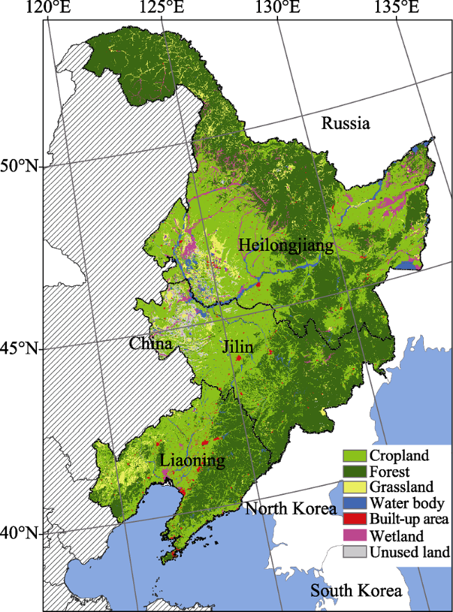
Figure 1 Land use in Northeast China in 2000. |
Table 1 List of input data used in this study |
| Variable | Description | Resolution | Source |
|---|---|---|---|
| Land use data | Remote sensing of land use patterns in 1990, 2000 and 2005 (including cropland, forest, grassland, water body, built-up area, wetland and unused land) | 1 km | Institute of Geographic Sciences and Natural Resources Research (IGSNRR), CAS |
| DEM | Spatial data, used to generate the aspect and slope | 1 km | IGSNRR, CAS |
| Temperature | Years average temperature; annual accumulated temperature ≥0℃; annual accumulated temperature ≥10℃ | 500 m | China Meteorological Administration |
| Rainfall | Years average rainfall | 1 km | China Meteorological Administration |
| Soil | Map; soil type (subclass) distribution | FAO soil classification | |
| Road | Level 1~3 traffic network distribution | National Fundamental GIS | |
| River | River water distribution | National Fundamental GIS | |
| Residential area | Residential distribution | National Fundamental GIS | |
| Population | Demographic data distribution map, 1 km grid, population: people/km2 | 1 km | IGSNRR, CAS |
| GDP | Data distribution diagram, 1 km grid, GDP unit: million yuan/km2 | 1 km | IGSNRR, CAS |
| Land use requirements | 7 land use types, provincial level, 1980-2010 | / | China Statistical Yearbooks |
Table 2 Settings of conversion elasticity |
| Simulation | Cropland | Forest | Grassland | Water body | Built-up area | Wetland | Unused land |
|---|---|---|---|---|---|---|---|
| Backward | 0.6 | 0.8 | 0.7 | 0.8 | 0.5 | 0.7 | 0.8 |
| Forward | 0.6 | 0.8 | 0.5 | 0.9 | 0.9 | 0.7 | 0.4 |
Table 3 β values of location factors in regression results related to each land use type; significant coefficients (P<0.05) are listed |
| Cropland | Forest | Grassland | Water body | Built-up area | Unused land | Wetland | |
|---|---|---|---|---|---|---|---|
| Constant | 47.08 | 18.38 | 90.53 | -181.19 | -2.55 | -111.15 | -82.06 |
| Aspect | 0.0015 | -0.0045 | 0.0028 | 0.0051 | -0.0020 | 0.0020 | 0.0038 |
| Elevation (DEM) | -0.0029 | 0.0025 | -0.0004 | -0.0076 | n.s. | 0.0040 | -0.0036 |
| GDP | 0.0008 | -0.0033 | 0.0034 | 0.0021 | 0.0126 | -0.0006 | -0.0034 |
| POP | 0.0076 | -0.0044 | -0.0043 | -0.0061 | 0.0023 | -0.0042 | -0.0022 |
| Rainfall | -0.0003 | 0.0006 | -0.0008 | n.s. | -0.0004 | -0.0011 | -0.0004 |
| Distance to residential area | 0.0006 | 0.0007 | 0.0022 | -0.0019 | -0.0030 | -0.0024 | 0.0020 |
| Distance to river | 0.0004 | 0.0007 | 0.0003 | -0.0034 | n.s. | 0.0030 | -0.0016 |
| Distance to road | n.s. | n.s. | n.s. | 0.0004 | 0.0004 | n.s. | n.s. |
| Slope | -0.0295 | 0.0565 | -0.0231 | -0.0310 | -0.0213 | -0.1249 | -0.0724 |
| Annual accumulated temperature ≥0℃ | -0.0539 | -0.0848 | -0.0772 | 0.3433 | n.s. | 0.3600 | -0.3730 |
| Annual accumulated t emperature ≥10℃ | 0.0066 | 0.0627 | -0.0100 | -0.1623 | n.s. | -0.2558 | 0.2983 |
| Annual mean temperature | 0.0271 | n.s. | 0.0301 | -0.0694 | n.s. | n.s. | 0.0218 |
| I-Bb-U-C (Soil_1) | 0.7175 | 0.3696 | -1.0162 | n.s. | n.s. | 3.3157 | 1.2644 |
| AO13-3bc (Soil_2) | -0.1009 | 1.3624 | -0.5527 | 0.3061 | 0.9438 | 4.2715 | n.s. |
| Ge63-2/3a (Soil_3) | 0.1418 | 0.6060 | 2.5921 | n.s. | n.s. | 1.8103 | n.s. |
| A080-2bc (Soil_4) | 1.0788 | n.s. | -0.5358 | 0.6740 | -1.1014 | 2.4519 | 1.0878 |
| I-Lo-2c (Soil_5) | 0.2481 | 0.4874 | 1.1863 | n.s. | n.s. | 2.9629 | n.s. |
| Kh1-2b (Soil_6) | 0.5820 | 0.9661 | n.s. | n.s. | 7.8537 | 6.0074 | n.s. |
| GL (Soil_7) | -0.8421 | 1.6314 | 2.3325 | n.s. | n.s. | n.s. | -5.0107 |
| Be87-2ab (Soil_8) | -0.3598 | 0.8706 | 2.8974 | n.s. | n.s. | n.s. | -3.4772 |
| Gm20-2/3a (Soil_9) | n.s. | 1.1289 | 0.1798 | 0.3058 | n.s. | 3.7156 | 0.6415 |
| I-K-2C (Soil_10) | -2.7090 | 1.8606 | -1.8423 | n.s. | 1.3232 | n.s. | 3.3136 |
| I-Y-2C (Soil_11) | 0.4994 | 0.4537 | n.s. | 0.5158 | n.s. | 7.6462 | 1.1321 |
| I-BH-U-C (Soil_12) | 0.5178 | 0.6890 | -0.4127 | 0.7754 | n.s. | 4.0914 | 0.9727 |
| Hg6-2/3a (Soil_13) | 0.3548 | -0.7586 | 0.9411 | 0.4694 | n.s. | 6.4765 | 0.5742 |
| J2-2a (Soil_14) | 2.3345 | n.s. | 0.9976 | -1.9142 | n.s. | 2.5272 | -1.7082 |
| Lg1-2b (Soil_15) | n.s. | -18.2998 | n.s. | 1.0302 | n.s. | n.s. | n.s. |
| Yh2-1b (Soil_16) | n.s. | n.s. | 0.8014 | 1.2989 | -0.3218 | 6.4905 | 1.4371 |
| I-Bh-2c (Soil_17) | n.s. | 0.3667 | n.s. | n.s. | n.s. | 5.9017 | 1.9701 |
| WAT (Soil_18) | -1.0158 | -0.6522 | -3.3175 | n.s. | 10.0656 | n.s. | 2.0486 |
| I-Xl-2c (Soil_19) | n.s. | n.s. | 1.4065 | 1.3493 | 1.1067 | 6.4157 | 0.8550 |
| I-B-U-2c (Soil_20) | -0.9316 | -1.2753 | -1.3537 | 3.9771 | 2.5932 | 5.5994 | n.s. |
| ROC | 0.93 | 0.95 | 0.82 | 0.94 | 0.98 | 0.97 | 0.90 |
Note: n.s., not significant at the 0.05 level |
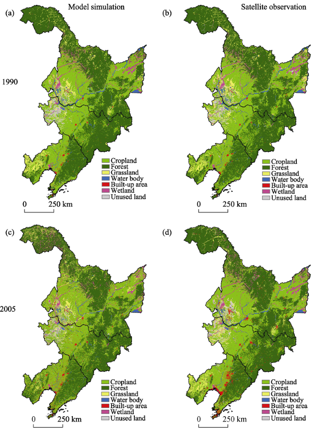
Figure 2 Comparison between model simulation (left) and satellite observation (right) in 1990 and 2005 |
Table 4 Conversion matrix between seven land use types (km2) |
| From To | Cropland | Forest | Grassland | Water body | Built-up area | Wetland | Unused land | Sum of decrease | |
|---|---|---|---|---|---|---|---|---|---|
| 1980 - 1990 | Cropland | - | 0 | 0 | 0 | 12 | 0 | 0 | 12 |
| Forest | 5468 | - | 0 | 11 | 0 | 0 | 5 | 5484 | |
| Grassland | 4394 | 0 | - | 0 | 214 | 0 | 0 | 4608 | |
| Water body | 758 | 0 | 0 | - | 0 | 0 | 0 | 758 | |
| Built-up area | 0 | 0 | 0 | 0 | - | 0 | 0 | 0 | |
| Wetland | 1231 | 6 | 7 | 0 | 9 | - | 0 | 1253 | |
| Unused land | 739 | 11 | 0 | 0 | 18 | 0 | - | 768 | |
| Sum of increase | 12590 | 17 | 7 | 11 | 241 | 0 | 5 | - | |
| 1990 - 2000 | Cropland | - | 5630 | 680 | 529 | 152 | 921 | 78 | 7990 |
| Forest | 9619 | - | 1003 | 208 | 8 | 752 | 113 | 11703 | |
| Grassland | 5896 | 283 | - | 58 | 58 | 35 | 2 | 6332 | |
| Water body | 1415 | 92 | 24 | - | 0 | 11 | 0 | 1542 | |
| Built-up area | 0 | 0 | 26 | 0 | - | 0 | 2 | 28 | |
| Wetland | 1015 | 31 | 2 | 17 | 1 | - | 15 | 1081 | |
| Unused land | 2632 | 196 | 0 | 0 | 4 | 0 | - | 2832 | |
| Sum of increase | 20577 | 6232 | 1735 | 812 | 223 | 1719 | 210 | - | |
| 2000 - 2010 | Cropland | - | 17140 | 5277 | 0 | 5711 | 360 | 1833 | 30321 |
| Forest | 7774 | - | 5275 | 0 | 4469 | 298 | 637 | 18453 | |
| Grassland | 6324 | 13757 | - | 0 | 907 | 0 | 4703 | 25691 | |
| Water body | 1428 | 162 | 280 | - | 0 | 588 | 26 | 2484 | |
| Built-up area | 22 | 1 | 6 | 0 | - | 0 | 3 | 32 | |
| Wetland | 9406 | 3068 | 4068 | 2 | 71 | - | 218 | 16833 | |
| Unused land | 1218 | 162 | 10181 | 0 | 669 | 110 | - | 12340 | |
| Sum of increase | 26172 | 34290 | 25087 | 2 | 11827 | 1356 | 7420 | - |
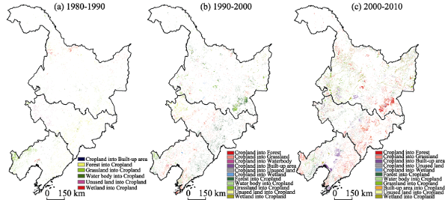
Figure 3 Spatio-temporal changes in cropland during the period 1980-1990 (a), 1990-2000 (b) and 2000-2010 (c) |
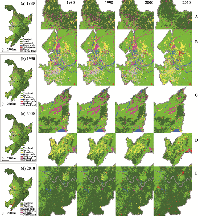
Figure 4 Simulated land use maps in 1980, 1990, 2000 and 2010 for five regions (A-E) |
The authors have declared that no competing interests exist.
| 1 |
|
| 2 |
|
| 3 |
|
| 4 |
|
| 5 |
|
| 6 |
|
| 7 |
|
| 8 |
|
| 9 |
|
| 10 |
|
| 11 |
|
| 12 |
|
| 13 |
|
| 14 |
|
| 15 |
|
| 16 |
|
| 17 |
|
| 18 |
|
| 19 |
|
| 20 |
|
| 21 |
|
| 22 |
|
| 23 |
|
| 24 |
|
| 25 |
|
| 26 |
|
| 27 |
|
| 28 |
|
| 29 |
|
| 30 |
|
| 31 |
|
| 32 |
|
| 33 |
|
| 34 |
|
| 35 |
|
| 36 |
|
| 37 |
|
| 38 |
|
| 39 |
|
| 40 |
|
| 41 |
|
| 42 |
|
| 43 |
|
| 44 |
|
| 45 |
|
| 46 |
|
| 47 |
|
| 48 |
|
| 49 |
|
| 50 |
|
| 51 |
|
/
| 〈 |
|
〉 |